
If you’ve read my earlier blogs centered on AutoML and machine learning on edge devices, you know how easy it is to train and test a custom ML model with little to no prerequisite knowledge.
However, just training an ML model isn’t enough. You also need to know how to use them to make predictions. Maybe you need to build a cross-platform app using tools like QT, or maybe you want to host your model on a server to serve requests via an API. This third blog in the series on training and running Tensorflow models in a Python environment covers just that!
Series Pit Stops
- Training a TensorFlow Lite Image Classification model using AutoML Vision Edge
- Creating a TensorFlow Lite Object Detection Model using Google Cloud AutoML
- Using Google Cloud AutoML Edge Image Classification Models in Python (You are here)
- Using Google Cloud AutoML Edge Object Detection Models in Python
- Running TensorFlow Lite Image Classification Models in Python
- Running TensorFlow Lite Object Detection Models in Python
- Optimizing the performance of TensorFlow models for the edge
Now, let’s take a closer look at how to use this model in Python.
Step 1: Exporting the trained model
Once a model has finished training, you can head over to Google Cloud and export the model to use it locally. You can do so by navigating to the “Test and Use” section of the dataset and choosing the option to export to a Docker container:
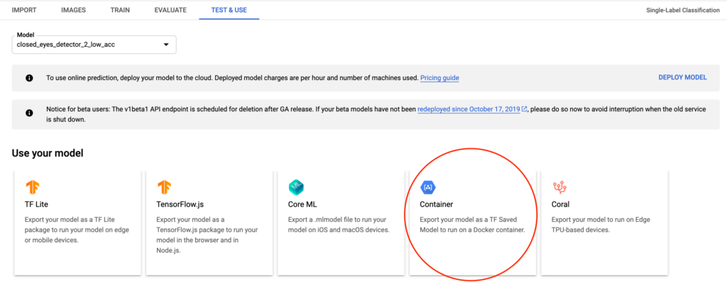
Doing so will result in a .pb file that you can download and use locally.
Step 2: Installing the required dependencies
Before we go ahead and write any code, it’s important that we first have all the required dependencies installed on our development machine.
For the current example, these are the dependencies we’ll need:
We can use pip to install these dependencies with the following command:
Step 3: Setting up the Python code for using the model
Now that we have the model and our development environment ready, the next step is to create a Python snippet that allows us to load this model and perform inference with it.
Here’s what such a snippet might look like:
# we want to run the inference on Tf 1.x instead of 2.x
import tensorflow.compat.v1 as tf
tf.disable_v2_behavior()

# path to the folder containing our downloaded .pb file
model_path = "/Users/harshitdwivedi/Desktop/downloaded_model"

# creating a tensorflow session (we will be using this to make our predictions later)
session = tf.Session(graph=tf.Graph())

# loading the model into our session created above
tf.saved_model.loader.load(session, ['serve'], model_path)
Try running the script above with the command python main.py, and if you don’t get any errors, you’re good to go!
Up next, we’ll be modifying the code above to read images from the local disk and load them into our ML model.
Step 4: Reading and providing input to the ML model
In this example, I’ll be using a model that I trained earlier, which tells me whether a provided image is underexposed or overexposed; so my trained model will essentially have 2 labels with which to classify input images.
To test if the model works as expected, I’ve placed a few images in a folder, and I’ll be passing the path of this folder and reading files from it in my code. Here’s how it can be done:
# we want to run the inference on Tf 1.x instead of 2.x
import tensorflow.compat.v1 as tf
tf.disable_v2_behavior()

import pathlib

# path to the folder containing our downloaded .pb file
model_path = "/Users/harshitdwivedi/Desktop/downloaded_model"

# path to the folder containing images
image_path = "/Users/harshitdwivedi/Desktop/Images"

# creating a tensorflow session (we will be using this to make our predictions later)
session = tf.Session(graph=tf.Graph())

# loading the model into our session created above
tf.saved_model.loader.load(session, ['serve'], model_path)

for file in pathlib.Path(image_path).iterdir():
  # get the current image path
  current_image_path = r"{}".format(file.resolve())

  # image bytes since this is what the ML model needs as its input
  img_bytes = open(current_image_path, 'rb').read()

  # pass the image as input to the ML model and get the result
  result = session.run('scores:0', feed_dict={
            'Placeholder:0': [img_bytes]})

  print("File {} has result {}".format(file.stem, result))
The code might look complex, but it’s actually not! Let’s break down it to see what’s happening here:
Lines 1–14: Initialization—discussed earlier.
Line 16: Here, we’re iterating through the directory in which the images are placed using PathLib.
Line 18–21: For each image, we convert it to a byte array, which is a format TensorFlow understands.
Line 24–27: For each byte array, we pass it to the session variable and get the output. scores:0 is the node in the model that stores the prediction scores; i.e. the output. Whereas the Placeholder:0 node is what stores the input.
If you run the code above and print the result, you’ll see something like this:
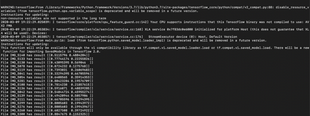
While we can see that TensorFlow does spew out some numbers, which look like probabilities—it’s a bit hard to make sense out of them at first glance.
Let’s see how we can format the output to human-readable results in the next step.
Step 5: Formatting the results obtained with TensorFlow
Since my image classification model was trained to detect 2 labels (under and overexposed images), it’s not a surprise that the resulting output array also has only 2 elements.
And naturally, each one of them belongs to the two labels I have in place.
To know which one is which, we can simply head over to the Dataset in the GCP console and navigate to the “Images” tab this time around.
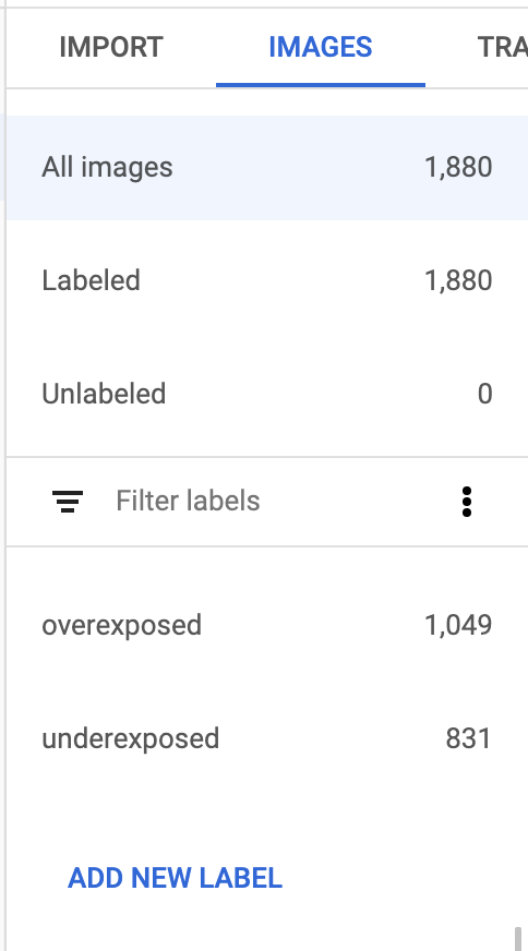
Overexposed is the first entry, followed by the underexposed entry; in our output array, the first entry is the probability that the given image is overexposed, and the second entry is the probability that the given image is underexposed.
So to convert this output into human-readable labels, we’ll simply get the largest value from the array (which corresponds to the highest probability) and map it to a label. This is how it can be done:
# we want to run the inference on Tf 1.x instead of 2.x
import tensorflow.compat.v1 as tf
tf.disable_v2_behavior()

import pathlib

# path to the folder containing our downloaded .pb file
model_path = "/Users/harshitdwivedi/Desktop/downloaded_model"

# path to the folder containing images
image_path = "/Users/harshitdwivedi/Desktop/Images"

# creating a tensorflow session (we will be using this to make our predictions later)
session = tf.Session(graph=tf.Graph())

# loading the model into our session created above
tf.saved_model.loader.load(session, ['serve'], model_path)

for file in pathlib.Path(image_path).iterdir():
  # get the current image path
  current_image_path = r"{}".format(file.resolve())

  # image bytes since this is what the ML model needs as its input
  img_bytes = open(current_image_path, 'rb').read()

  # pass the image as input to the ML model and get the result
  result = session.run('scores:0', feed_dict={
            'Placeholder:0': [img_bytes]})

  probabilities = result[0]

  if probabilities[0] > probabilities[1]:
    # the first element in the array is largest
    print("Image {} is OverExposed".format(file.stem))
  else:
    # the second element in the array is largest
    print("Image {} is UnderExposed".format(file.stem))
Now, on running the code again, this is what we see:
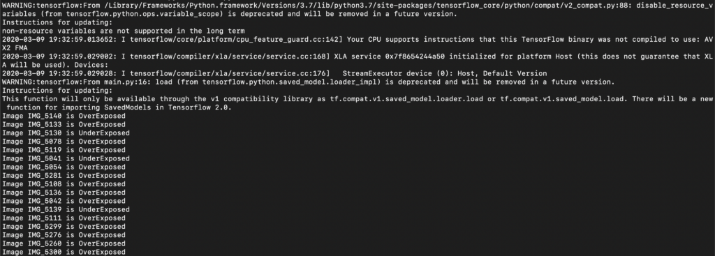
Notice how the output is now formatted to human-readable labels instead.
And that’s it! We can further extend this code snippet to display the images the model is detecting using OpenCV, and then moving the images to different folders based on their labels.
In the next part of this post, I’ll be covering how we can do the same for object detection models to track and draw the detected objects on an image. Stay tuned for that!
Thanks for reading! If you enjoyed this story, please click the 👏 button and share it to help others find it! Feel free to leave a comment 💬 below.
Have feedback? Let’s connect on Twitter.

Comments 0 Responses