
This blog is the fourth one in my series on training and running Tensorflow models in a Python environment. If you haven’t read my earlier blogs centered on AutoML and machine learning on edge devices, I’d suggest that you do so before continuing with this post.
Training a model this easily is great, but we also need to know how to use it to make predictions. For example, if you want to build a desktop app that uses TensorFlow for machine learning, or maybe a website that allows users to upload an image and identify matching apparel to the one found in the image. This blog outlines just that—how you can use these edge models in a Python environment.
Step 1: Exporting the trained model
Once a model has finished training, you can head over to Google Cloud and export the model to use it locally. You can do so by navigating to the “Test and Use” section of the dataset and choosing the option to export to a Docker container:
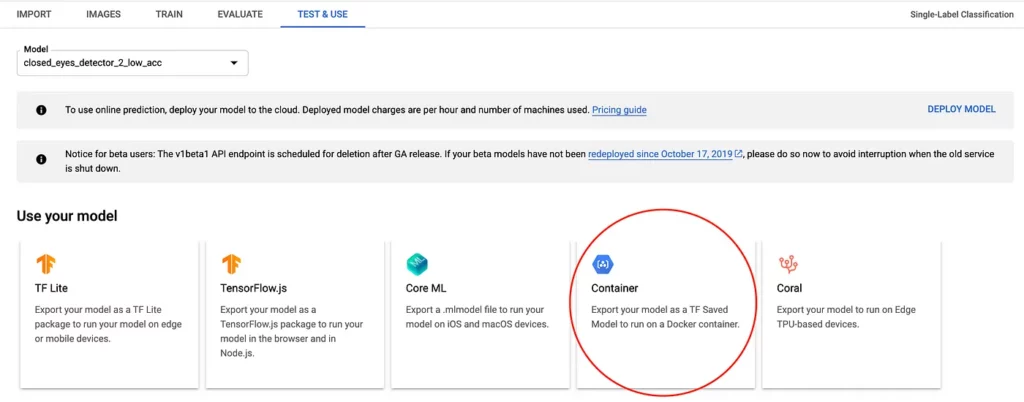
Doing so will result in a .pb file that you can download and use locally. Once downloaded, rename the file to saved_model.pb.
Step 2: Installing the required dependencies
Before we go ahead and write any code, it’s important that we first have all the required dependencies installed on our development machine.
For the current example, these are the dependencies that we’ll need:
We can use pip to install these dependencies by the following command:
Step 3: Setting up the Python code for using the model
Now that we have the model and our development environment ready, the next step is to create a Python snippet that allows us to load this model and perform inference with it.
Here’s what such a snippet might look like:
# we want to run the inference on Tf 1.x instead of 2.x
import tensorflow.compat.v1 as tf
tf.disable_v2_behavior()

# path to the folder containing our downloaded .pb file
model_path = "/Users/harshitdwivedi/Desktop/downloaded_model"

# creating a tensorflow session (we will be using this to make our predictions later)
session = tf.Session(graph=tf.Graph())

# loading the model into our session created above
tf.saved_model.loader.load(session, ['serve'], model_path)
Try running the script above with the command python main.py, and if you don’t get any errors, you’re good to go!
Up next, we’ll be modifying the code above to read images from the local disk and load them into our ML model.
Step 4: Reading and providing input to the ML model
In this example, I’m using a model that I trained earlier, which detects and provides the bounding box for humans present in a given image.
To test if the model works as expected, I’ve placed a few images in a folder, and I’ll be passing the path of this folder and reading files from it in my code. Here’s how it can be done:
# we want to run the inference on Tf 1.x instead of 2.x
import tensorflow.compat.v1 as tf
tf.disable_v2_behavior()

import pathlib

# path to the folder containing our downloaded .pb file
model_path = "/Users/harshitdwivedi/Desktop/downloaded_model"

# path to the folder containing images
image_path = "/Users/harshitdwivedi/Desktop/Images"

# creating a tensorflow session (we will be using this to make our predictions later)
session = tf.Session(graph=tf.Graph())

# loading the model into our session created above
tf.saved_model.loader.load(session, ['serve'], model_path)

for file in pathlib.Path(image_path).iterdir():
  # get the current image path
  current_image_path = r"{}".format(file.resolve())

  # image bytes since this is what the ML model needs as its input
  img_bytes = open(current_image_path, 'rb').read()

  # pass the image as input to the ML model and get the result
  boxes = session.run(['detection_boxes:0','detection_scores:0'], feed_dict={
            'encoded_image_string_tensor:0': [img_bytes]})

  print("File {} has result {}".format(file.stem, boxes))
While the rest of the code looks similar to the blog post covering image classification models, this time around the result and the input/output tensors are different.
In the snippet above, since we’re working with an object detection model, we want not only the scores but also the coordinates to determine where to draw the bounding box; hence, the output is a list of two tensors in the run() method.
On running the code above, this is what you might see printed on the screen:
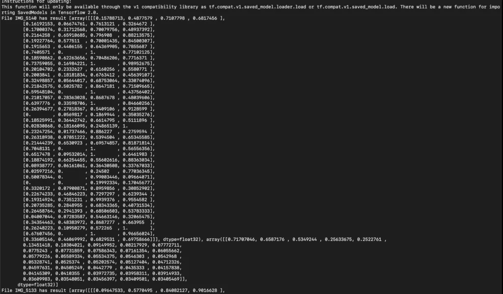
Unlike with image classification, the output is a bit harder to make sense of; but worry not. Let’s try to see what these numbers mean in the next section.
Step 5: Understanding the results obtained with TensorFlow
As we can see in the output above; the result is an array that internally holds 2 arrays (Arrayception!).
The first array here corresponds to the first entry in our run() method’s input (detection_boxes), while the second array corresponds to the second entry in the run method’s output (detection_scores).
If you switch these two tensors in the list; you’ll see the position of these two arrays flipped in the output!
Now that we know that the first array holds the coordinates of the detected object, let’s count the items it has detected in the image.
The following statement should tell us just that:
If everything works as expected, you should see an integer printed that determines the number of objects detected by the ML model.
For me, it came out as 40.
Now if you try to print the number of scores, it should be the same:
What does this tell us? It means that the second array contains the scores for each of the boxes the model detected and provided in the first array.
Now, it’s obvious that not all the detected objects are of use—since my image doesn’t even have 40 objects in it! For your reference; this is the image that I used:

To identify only the objects with a high enough accuracy, let’s filter the results to only contain objects with a probability higher than 25%. This is how we can do so:
# we want to run the inference on Tf 1.x instead of 2.x
import tensorflow.compat.v1 as tf
tf.disable_v2_behavior()
import pathlib
# path to the folder containing our downloaded .pb file
model_path = "/Users/harshitdwivedi/Downloads"
# path to the folder containing images
image_path = "/Users/harshitdwivedi/Desktop/Archive 2"
# creating a tensorflow session (we will be using this to make our predictions later)
session = tf.Session(graph=tf.Graph())
# loading the model into our session created above
tf.saved_model.loader.load(session, ['serve'], model_path)
for file in pathlib.Path(image_path).iterdir():
# get the current image path
current_image_path = r"{}".format(file.resolve())
# image bytes since this is what the ML model needs as its input
img_bytes = open(current_image_path, 'rb').read()
# pass the image as input to the ML model and get the result
result = session.run(['detection_boxes:0', 'detection_scores:0'], feed_dict={'encoded_image_string_tensor:0': [img_bytes]})
boxes = result[0][0]
scores = result[1][0]
print("For file {}".format(file.stem))
for i in range(len(scores)):
# only consider a detected object if it's probability is above 25%
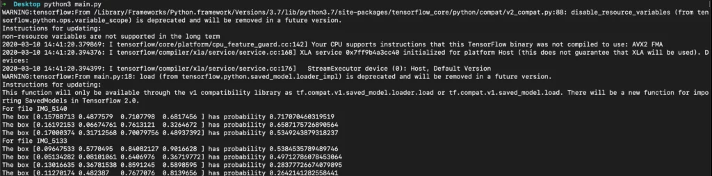
if scores[i] > 0.258:
print("The box {} has probability {}".format(boxes[i], scores[i]))Now, once you run this code snippet, the output should be much more intuitive:
Perfect! Now that we understand the output, let’s see how to plot these coordinates on an image to see how the ML model actually performs.
Step 6: Using OpenCV to draw coordinates on the image and visualize the output
Using OpenCV, we can not only view the image being processed, but we can also draw various shapes on it. We’ll use this OpenCV feature to our advantage here and draw the detected boxes on the image.
Here’s the code snippet outlining how you can do this:
# we want to run the inference on Tf 1.x instead of 2.x
import tensorflow.compat.v1 as tf
tf.disable_v2_behavior()
import cv2
import pathlib

# path to the folder containing our downloaded .pb file
model_path = "/Users/harshitdwivedi/Downloads"

# path to the folder containing images
image_path = "/Users/harshitdwivedi/Desktop/Archive 2"

# creating a tensorflow session (we will be using this to make our predictions later)
session = tf.Session(graph=tf.Graph())

# loading the model into our session created above
tf.saved_model.loader.load(session, ['serve'], model_path)

# extract the coordinates of the rectange that's to be drawn on the image
def draw_boxes(height, width, box, img):
  # starting coordinates of the box
  ymin = int(max(1, (box[0] * height)))
  xmin = int(max(1, (box[1] * width)))
  # last coordinates of the box
  ymax = int(min(height, (box[2] * height)))
  xmax = int(min(width, (box[3] * width)))

  # draw a rectange using the coordinates
  cv2.rectangle(img, (xmin, ymin), (xmax, ymax), (10, 255, 0), 10)

for file in pathlib.Path(image_path).iterdir():
  # get the current image path
  current_image_path = r"{}".format(file.resolve())

  # image bytes since this is what the ML model needs as its input
  img_bytes = open(current_image_path, 'rb').read()

  # pass the image as input to the ML model and get the result
  result = session.run(['detection_boxes:0', 'detection_scores:0'], feed_dict={'encoded_image_string_tensor:0': [img_bytes]})

  boxes = result[0][0]
  scores = result[1][0]

  print("For file {}".format(file.stem))

  # read the image with opencv
  img = cv2.imread(current_image_path)
  # get the width and height of the image
  imH, imW, _ = img.shape

  for i in range(len(scores)):
    # only consider a detected object if it's probability is above 25%
    if scores[i] > 0.258:
      print("The box {} has probability {}".format(boxes[i], scores[i]))
      draw_boxes(imH, imW, boxes[i], img)

  # resize the image to fir the screen
  new_img = cv2.resize(img, (1080, 1920))
  # show the image on the screen
  cv2.imshow("image", new_img)
  # as soon as any key is pressed, skip to the next line
  cv2.waitKey(0)
And that’s it!
Upon running the complete code snippet above, you should be able to see outputs as follows:

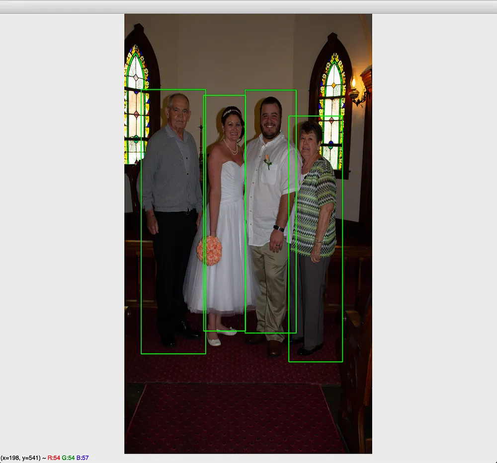
As you can see, the trained model was able to identify and draw bounding boxes around humans it has detected in the image.
If you aren’t happy with the accuracy of the trained model, you can either retrain it or play around with the accuracy threshold to get better performance.
(Optional) Step 7: Batching the inference for faster results
If you want even faster results, you might consider batching the calls made to session.run with multiple images in one go!
However, that being said; the object detection model will expect all your images to have the same dimension if you are to batch them.
Here’s a sample code that outlines how to batch the requests made to my model:
def main():
  images = []
  file_names = []
  for file in pathlib.Path("images")
    # resize the images to all have the same size
    image = get_resized__image(file.resolve(),512, 512)
    images.append(image)
    # save the current file name
    file_names.append(file.stem)

  # once all the images have been collected for batching, run the object detection
  detect_humans(images, file_names)

def get_resized__image(image_path, width, height):
    file = r"{}".format(image_path)
    im = Image.open(file)
    im_resize = im.resize((width, height))
    buf = io.BytesIO()
    im_resize.save(buf, format='JPEG')
    byte_im = buf.getvalue()
    return byte_im

def detect_humans(self, binary_images, file_names):
        human_results = []
        batch_result = self.session_human.run(['detection_boxes:0', 'detection_scores:0'], feed_dict={
            'encoded_image_string_tensor:0': binary_images})

        print("Batch result is {}".format(batch_result[0]))

        # all the boxes detected in all the images
        result_boxes = batch_result[0]
        # all the scores for all the boxes
        result_scores = batch_result[1]

        # iterate through all the boxes
        for index, result_box in enumerate(result_boxes):
            # box and score for the current image
            boxes = result_box
            scores = result_scores[index]

            print("Boxes for file {} are {}".format(file_names[index], boxes))
            print("Scores for the file {} are {}".format(file_names[index], scores))

            # draw boxes as shown in the code above
However, do note that setting a very large batch size might cause out of memory errors and your app might crash! So keep this in mind while batching your requests and be conservative with your batch sizes 🙂
And that’s it! We can further extend this code snippet to detect multiple objects and use OpenCV to draw their bounding boxes in different colors if needed (i.e. detect people and flowers). You can also modify the code above to extract the detected objects from the and image and save it as a new image altogether!
In the next part of this post, I’ll be covering the ways to improve the performance of your ML models by allowing them to perform more inference in less time while using lesser system resources, so stay tuned for that!
Thanks for reading! If you enjoyed this story, please click the 👏 button and share it to help others find it! Feel free to leave a comment 💬 below.
Have feedback? Let’s connect on Twitter.

Comments 0 Responses