
Human thoughts are persistent, and this enables us to understand patterns, which in turn gives us the ability to predict the next sequence of actions. Your understanding of this article will be based on the previous words that you’ve read. Recurrent Neural Networks replicate this concept.
RNNs are a type of artificial neural network that are able to recognize and predict sequences of data such as text, genomes, handwriting, spoken word, or numerical time series data. They have loops that allow a consistent flow of information and can work on sequences of arbitrary lengths.
Using an internal state (memory) to process a sequence of inputs, RNNs are already being used to solve a number of problems:
- Language translation and modeling
- Speech recognition
- Image captioning
- Time series data such as stock prices to tell you when to buy or sell
- Autonomous driving systems to anticipate car trajectories and help avoid accidents.
I’ve written this with the assumption that you have a basic understanding of neural networks. In case you need a refresher, please go through this quick Introduction to Neural Networks.
Understanding Recurrent Neural Networks.
To understand RNNs, let’s use a simple perceptron network with one hidden layer. Such a network works well with simple classification problems. As more hidden layers are added, our network will be able to inference more complex sequences in our input data and increase prediction accuracy.
RNN Structure
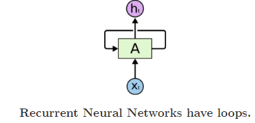
A — Neural Network.
Xt- Input.
ht — Output.
Loops ensure a consistent flow of information. A (chunk of neural network) produces an output ht based on the input Xt .
RNNs can also be viewed as multiple copies of the same network, each passing information to its successor.
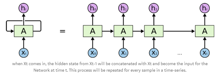
At each time step (t), the recurrent neuron receives the input Xt as well as its own output from the previous time step ht-1.
There are a number of great resources if you would like to dive deeper into RNNs, which I strongly recommend. They include:
Introduction to Recurrent Neural Networks.
Recurrent Neural Networks for Beginners.
RNNs have a major setback called vanishing gradient; that is, they have difficulties in learning long-range dependencies (relationship between entities that are several steps apart).
Imagine we have the price of bitcoin for December 2014, which was say $350, and we want to correctly predict the bitcoin price for the months of April and May 2018. Using RNNs, our model won’t be able to predict the prices for these months accurately due to the long range memory deficiency. To solve this issue, a special kind of RNN called Long Short-Term Memory cell (LSTM) was developed.
What is a Long Short-Term Memory Cell?
This is a special neuron for memorizing long-term dependencies. LSTM contains an internal state variable which is passed from one cell to the other and modified by Operation Gates (we’ll discuss this later in our example).
LSTM is smart enough to determine how long to hold onto old information, when to remember and forget, and how to make connections between old memory with the new input. For an in-depth understanding of LSTMs, here is a great resource: Understanding LSTM networks.
Implementing LSTMs
In our case, we’re going to implement a time series analysis using LSTMs to predict the prices of bitcoin from December 2014 to May 2018. I have used the historical data from CryptoDataDownload since I found it simple and straightforward. I used google’s Colab development environment because of the simplicity in setting up the environment and the accelerated free GPU, which eases the training time for my model. If you are new to Colab, here’s a beginner’s guide. The bitcoin .csv file and the entire code for this example can be obtained from my github profile.
What is time series analysis?
This is where historical data is used to identify existing data patterns and use them to predict what will happen in the future. For a detailed understanding, refer to this guide.
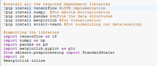
Importing libraries
We’re going to work with a variety of libraries that we’ll have to install first in our Colab notebook and then import into our environment.
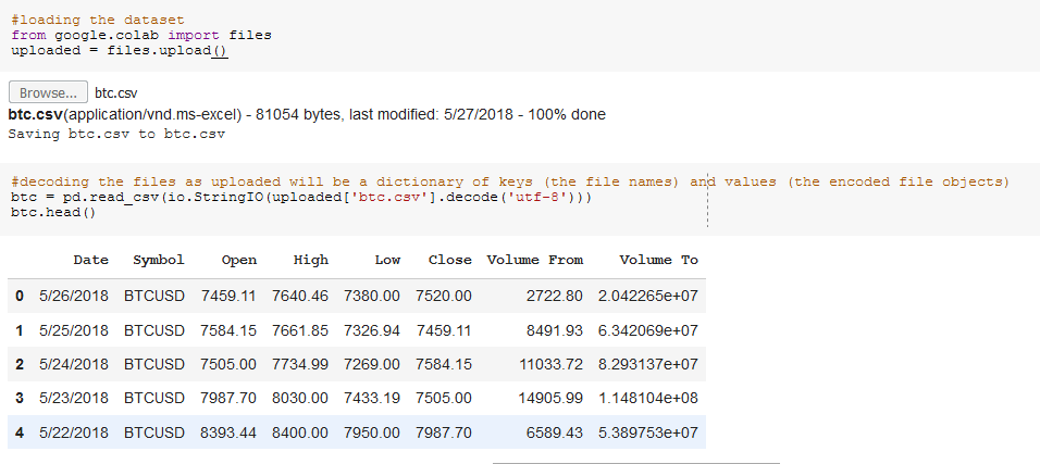
Loading the dataset
The btc.csv dataset contains the prices and volumes of bitcoin, and we load it into our working environment using the following commands:
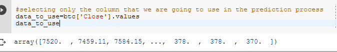
Target Variable
We are going to select the bitcoin closing price as our target variable to predict.
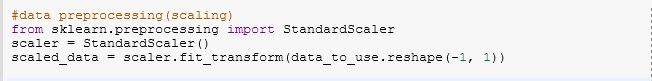
Data preprocessing
Sklearn contains the preprocessing module that allows us to scale our data and then fit it in our model.
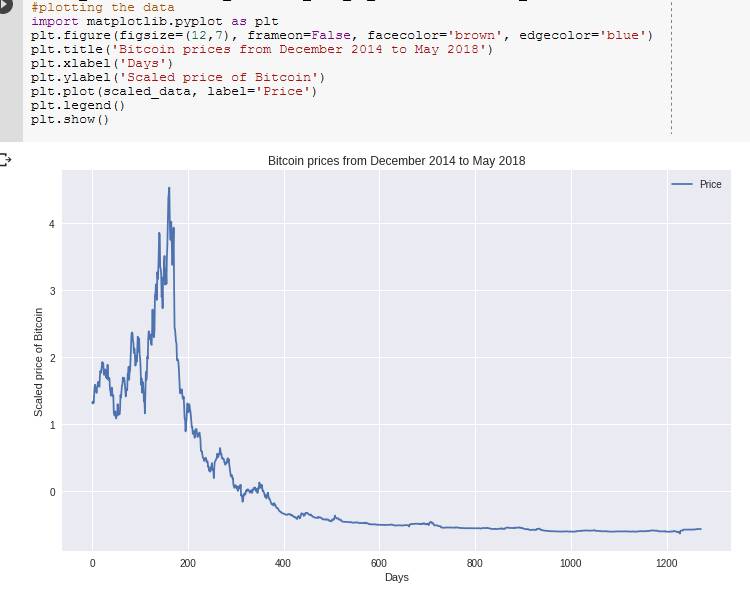
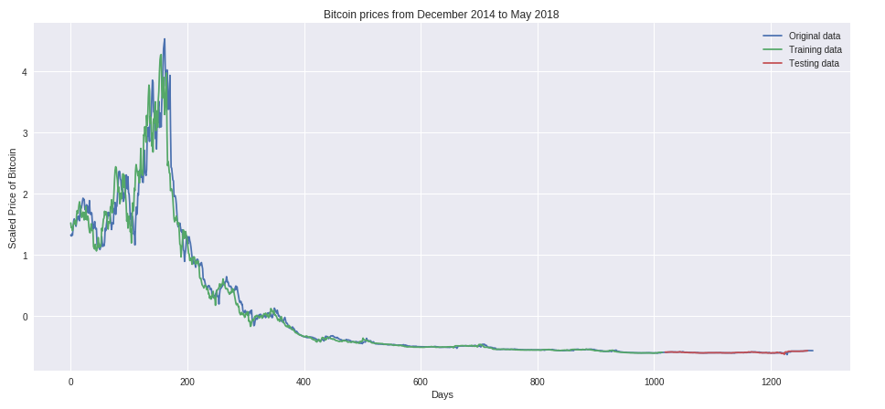
Plotting our data
Let’s now take a look at how the bitcoin close price trended over the given time period.
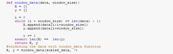
Features and label dataset
This function is used to create the features and labels for our data set by windowing the data.
Input: data — this is the dataset we are using .
Window_size — how many data points we are going to use to predict the next datapoint in the sequence. (Example if window_size=7 we are going to use the previous 7 days to predict the bitcoin price for today).
Outputs: X — features split into windows of data points(if windows_size=1, X=[len(data)-1,1]).
y — labels — this is the next number in the sequence that we’re trying to predict.
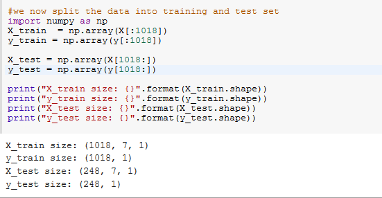
Training and Testing dataset
Splitting the data into training and test sets is crucial for getting a realistic estimate of our model’s performance. We have used 80% (1018) of the dataset as the training set and the remaining 20% (248) as the validation set.
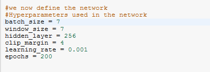
Defining the network
Hyperparameters
Hyperparameters explain higher-level structural information about a model.
batch_size — This is the number of windows of data we are passing at once.
window_size — The number of days we consider to predict the bitcoin price for our case.
hidden_layers — This is the number of units we use in our LSTM cell.
clip_margin — This is to prevent exploding the gradient — we use clipper to clip gradients below above this margin.
learning_rate — This is a an optimization method that aims to reduce the loss function.
epochs — This is the number of iterations (forward and back propagation) our model needs to make.
There are a variety of hyperparameters that you can customize for your model, but for our example let’s stick to those we’ve defined.
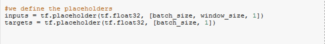
Placeholders
Placeholders allows us to send different data within our network with the tf.placeholder() command.
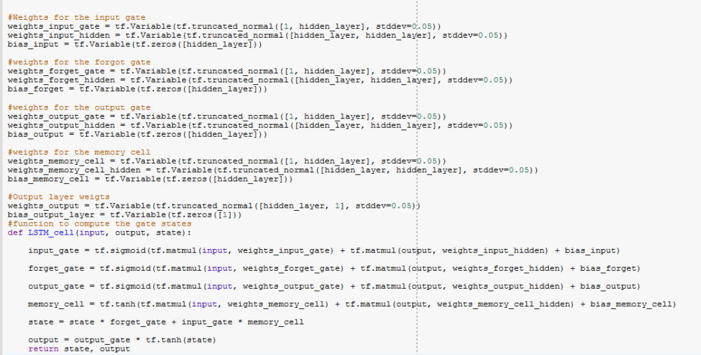
LSTM Weights
LSTM weights are determined by Operation Gates which include: Forget, Input and Output gates.
Forget Gate
ft =σ(Wf[ht-1,Xt]+bf)
This is a sigmoid layer that takes the output at t-1 and the current input at time t and then combines them into a single tensor. It then applies linear transformation followed by a sigmoid.
The output of the gate is between 0 and 1 due to the sigmoid. This number is then multiplied with the internal state, and that is why the gate is called forget gate. If ft =0 ,then the previous internal state is completely forgotten, while if ft =1, it will be passed unaltered.
Input Gate
it=σ(Wi[ht-1,Xt]+bi)
This state takes the previous output together with the new input and passes them through another sigmoid layer. This gate returns a value between 0 and 1. The value of the input gate is then multiplied with the output of the candidate layer.
Ct=tanh(Wi[ht-1,Xt]+bi)
This layer applies hyperbolic tangent to the mix of the input and previous output, returning the candidate vector. The candidate vector is then added to the internal state, which is updated with this rule:
Ct=ft *Ct-1+it*Ct
The previous state is multiplied by the forget gate, and then added to the fraction of the new candidate allowed by the output gate.
Output Gate
Ot=σ(Wo[ht-1,Xt]+bo)
ht=Ot*tanh Ct
This gate controls how much of the internal state is passed to the output and works in a similar manner to the other gates.
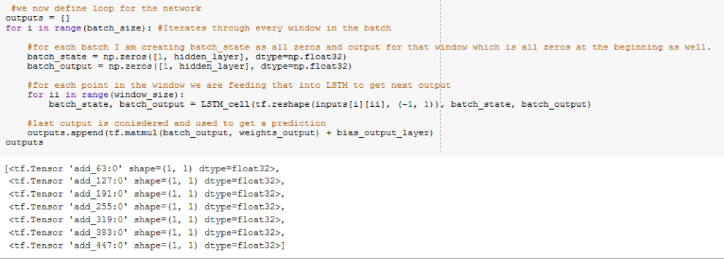
Network loop
A loop for the network is created which iterates through every window in the batch creating the batch_states as all zeros .The output is the used for predicting the bitcoin price.
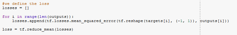
Defining the loss
Here we will use the mean_squared_error function for the loss to minimize the errors.
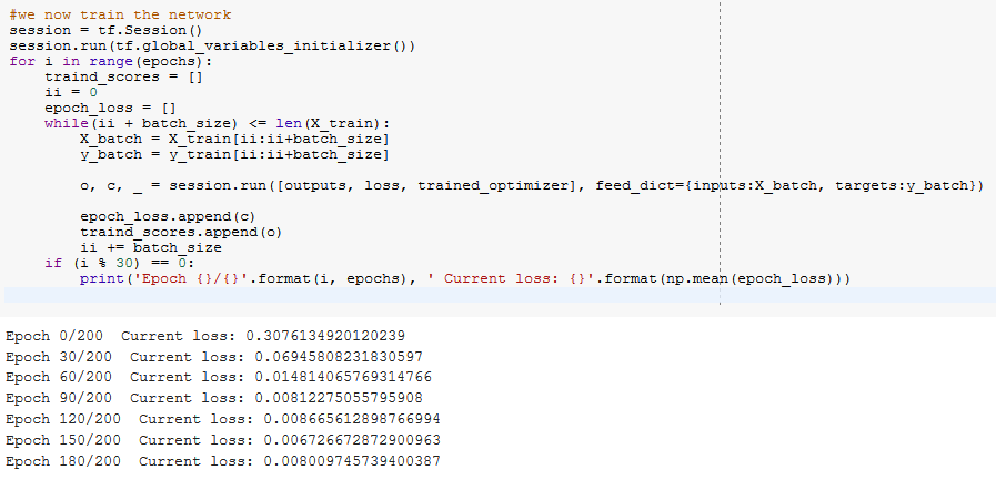
Training the network
We now train the network with the number of epochs (200), which we had initialized, and then observe the change in our loss through time. The current loss decreases with the increase in the epochs as observed, increasing our model accuracy in predicting the bitcoin prices.
Plotting the predictions
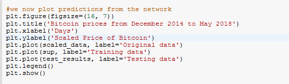
Output
Our model has been able to accurately predict the bitcoin prices based on the original data by implementing LSTMs cells. We could improve the model performance by reducing the window length from 7 days to 3 days. You can tweak the full code to optimize your model performance.
Conclusion.
I was inspired by this blog on using LSTMs for time series analysis. I would recommend it to gain more insights. Also check out this look at using an LSTM as a foundation for predicting stock prices over time
I hope this article has given you a head start in understanding LSTMs. Feel free to comment, clap, and share.
Discuss this post on Hacker News.
Comments 0 Responses