Working with Geospatial Data in Machine Learning

In data science competitions and machine learning projects, we often may encounter geospatial features that are (most of the time) represented as longitude and latitude.

These kinds of features will influence your predictive model’s results by a large margin if they aren’t well represented; therefore, these features are seldom considered, and they’re often eliminated from the feature’s set.

In this article, we’ll show you how to work with this type of data—first by visualizing them to obtain valuable insights; then, we’ll show you different methods you can use to extract and design new features that will improve your model.

Environment Setup

We’ll be using Anaconda with Python 3.6 as our environment for this demonstration, in which a lot of libraries are pre-installed, such as Pandas, NumPy and Matplotlib.

Besides these pre-installed libraries, we’ll also need the followings:

• Geopy for geocoding and reverse geocoding.
• Folium to display maps with coordinates and markers.

Here is how you can install them in your environment using pip or conda:

We can use any dataset that has longitude or latitude attributes, but here’s a Kaggle dataset that will satisfy our curiosity.

For this article, let’s suppose that I have a DataFrame called train that, among other features, includes Pickup Long and Pickup Lat. This will be the dataset used for testing.

Visualization

In data science, data visualization is a paramount task that engineers start with.

Their aim is to find and gather some insights to help build the best model possible for the task at hand. Here are a few of those potential insights, particular to geospatial data:

• Detecting, outliers, patterns, and trends.
• Contextualizing data in the real world.
• Understanding the distribution of data across cities, states, or countries.
• See how the data looks in general.

With these insights, we can make critical decisions to keep these features or remove them. To gather these insights, we’ll draw a number of plots.

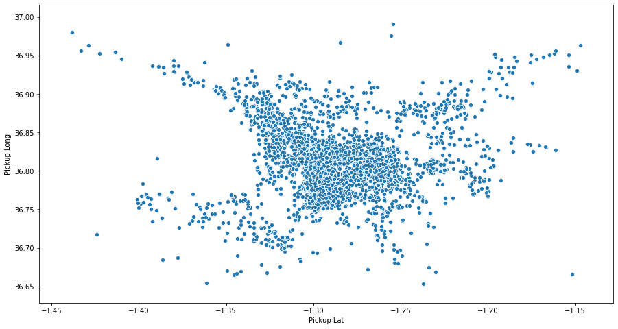
Scatter Plot

The fastest way to visualize our geospatial data is through a scatter plot, which basically shows the points in relation to each other. To display such a plot, you can use Matplotlib’s scatter plot or Seaborn’s. Here’s an example:

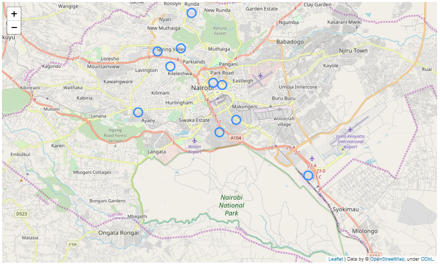
Map Plot

The second technique is to plot the data on a real map. This is a more obvious and real-world way to display coordinates and investigate the data.

There are a lot of libraries that offer such functionality, but we’ll be using the folium library, which we installed at the beginning.

Using the folium library is fairly straightforward:

1. Create a map with a location that can be the center point of your data.
2. Add the points to the map.
3. Display the map.

Here’s a sample implementation:

import folium

# create the map.
map_pickup = folium.Map( location=[-1.317755,36.830370])

# adding the latitude and longitude points to the map.
train.apply(lambda row:folium.CircleMarker(location=[row["Pickup Lat"], row["Pickup Long"]] ).add_to(map_pickup), axis=1)

# display the map: just ask for the object representation in juypter notebook.
map_pickup

# optional: save the map.
map_pickup.save('map_pickup.html')

And here’s what we got after only displaying 10 points:

Techniques & Ideas

After seeing what the data looks like, it’s time to shed some light on the feature engineering phase. Here, we’ll explore some ideas and techniques to extract and build better features that will improve our predictive model.

1- Use features as they are

The first thought that comes to mind is to use longitude and latitude as they currently are in the predictive model.

But bear in mind that the scale of the two variables is different, so you need to use a model that doesn’t require any normalization, like tree-based algorithms. Otherwise, you’ll have to perform normalization and include them in the feature set.

You can take this a step further by using a model that doesn’t need any normalization. Instead, you can just round the features to 3 or 4 decimal places, which will improve your model’s performance. Here’s how we can do this in pandas:

Another simple but powerful transformation is to convert the latitude and longitude to radians instead of degrees. This will basically represent the same thing but in a different unit. You can achieve that using the NumPy function radians().

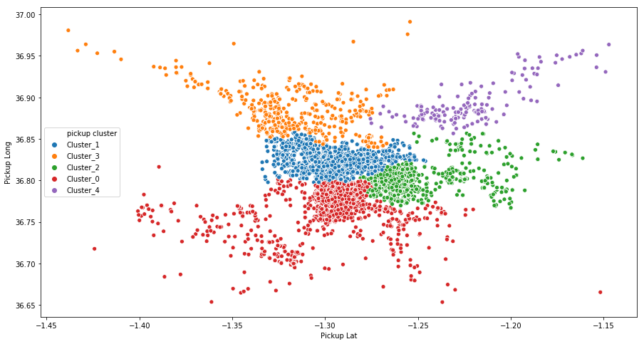
2- Perform Clustering

One of the approaches to handle point coordinates is to treat them in relation to each other.

In order to do that, we perform clustering and then assign each cluster-id to a point. By doing this, we’ll create a categorical variable that we can one hot encode to get better results.

The choice of the clustering algorithm matters. I tested many algorithms like K-means, DBSCAN, and hierarchical clustering—the latter two seem to give better results when it comes to geospatial features.

This is true given that K-means works well when trying to maximize variance, which is good if the feature space is linear in nature. But if it’s non-linear, then hierarchical clustering and DBSCAN are the best choices.

The number of clusters will depend on the problem, but in general, we have to test and see what gives better results.

Here is a sample that illustrates using K-means and hierarchical clustering algorithms with 5 clusters each:

from sklearn.cluster import KMeans ,AgglomerativeClustering

# creates 5 clusters using hierarchical clustering.
agc = AgglomerativeClustering(n_clusters =5, affinity='euclidean', linkage='ward')
train['pickup cluster'] = agc.fit_predict(train[['Pickup Lat','Pickup Long']])

# creates 5 clusters using k-means clustering algorithm.
kmeans = KMeans(5)
clusters = kmeans.fit_predict(train[['Pickup Lat','Pickup Long']])
train['pickup cluster'] = kmeans.predict(train[['Pickup Lat','Pickup Long']])

If we re-plot the data using the newly created clusters, we obtain the following plot:

3- Reverse Geocoding

It often happens that the point’s coordinates are far enough from each other and the data rows contain coordinates from different cities or countries in the world.

We can make use of this fact to perform reverse geocoding, which basically converts point coordinates to a readable address or place name (i.e. cities or countries). That way, we can create a new categorical variable.

from geopy.geocoders import Nominatim

# create the locator
geolocator = Nominatim(user_agent="myGeocoder")

# getting the location address
location = geolocator.reverse("52.509669, 13.376294")
print(location)
# >>> result : Backwerk, Potsdamer Platz, Tiergarten, Mitte, Berlin, 10785, Deutschland

# getting address compontent like street, city, state, country, country code, postalcode and so on.
location.raw.get('address').get('state')
location.raw.get('address').get('city_district')
location.raw.get('address').get('country')
location.raw.get('address').get('postcode')

And from that, we can create a field for city or country, but in some cases, where the measured points are in the same city, that method won’t work well— it will create a city variable with only one unique value.

For that, you have to extract the street or something else that varies from point to point.

4- Distance Feature:

To demonstrate this next technique, let’s consider the problem of determining ETA (Estimated Time of Arrival). For this, the dataset will contain departure and arrival coordinates.

From that, you can create a distance feature. This will improve your model a lot if the problem relies on the said feature—and ETA problems are very much in this category.

If you don’t have two coordinates, you can calculate the distance to a fixed point (e.g origin), which will depend on the context of your problem.

The distance formula we use here is the Harvsine Formula, which takes into consideration that the earth’s shape is a sphere and not flat, so the distance is more realistic.

Here’s an implementation of the Harvsine Formula and its application on our dataset:

import numpy as np

def haversine_distance(row):
    lat_p, lon_p = row['Pickup Lat'], row['Pickup Long']
    lat_d, lon_d = row['Destination Lat'], row['Destination Long']
    radius = 6371 # km

    dlat = np.radians(lat_d - lat_p)
    dlon = np.radians(lon_d - lon_p)
    a = np.sin(dlat/2) * np.sin(dlat/2) + np.cos(np.radians(lat_p)) * np.cos(np.radians(lat_d)) * np.sin(dlon/2) * np.sin(dlon/2)
    c = 2 * np.arctan2(np.sqrt(a), np.sqrt(1-a))
    distance = radius * c

    return distance

train['distance'] = train.apply(haversine_distance, axis = 1)

5- Extract X, Y, and Z:

I found this method on the data science stack exchange platform. It can moderately help our model but might be less effective than the previous methods.

The idea here is to represent those latitudes and longitudes via 3 coordinates. The problem with latitude and longitude is that they’re 2 features that represent a 3-dimensional space. We can, however, extract X, Y, and Z (our 3rd dimension) using sin and cosine functions. In this way, these features can be normalized properly.

The rule to derive these coordinates is the following:

Here is the Python code we need to apply on our dataset:

import numpy as np

train['pickup x'] = np.cos(train['Pickup Lat']) * np.cos(train['Pickup Long'])
train['pickup y'] = np.cos(train['Pickup Lat']) * np.sin(train['Pickup Long'])
train['pickup z'] = np.sin(train['Pickup Lat'])

6- Other derived features

Besides all the aforementioned features that you can extract from geospatial data, you can handcraft some more with the following ideas:

1. Nearest city name
2. Distance to the nearest city
3. Nearest city population
4. Nearest big city
5. Distance to the nearest big city

These features include populations, city names, and distances—and they require a lot of code.

Resources

• Here is an article about the visualization of geospatial data.
• For more information about the geopy library, check out the official docs.
• To customize the map we showed, check out the official folium documentation for more details.
• Don’t forget to see all the clustering algorithms that the sklearn library offers.

Feature engineering is an art rather than a science, in which creativity plays an important role. This is especially true when we deal with features that are naturally difficult for machine learning models to predict with. As such, we have to deal carefully with it—that’s why feature engineering is a critical step to undertake in such a case.