Working with Audio Data for Machine Learning in Python

Most of the attention, when it comes to machine learning or deep learning models, is given to computer vision or natural language sub-domain problems.

However, there’s an ever-increasing need to process audio data, with emerging advancements in technologies like Google Home and Alexa that extract information from voice signals. As such, working with audio data has become a new trend and area of study.

The possible applications extend to voice recognition, music classification, tagging, and generation, and are paving the way for audio use cases to become the new era of deep learning.

Audio File Overview

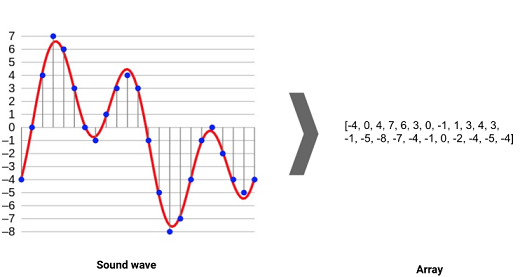
Sound are pressure waves, and these waves can be represented by numbers over a time period. These air pressure differences communicates with the brain. Audio files are generally stored in .wav format and need to be digitized, using the concept of sampling.

Loading and Visualizing an audio file in Python

Librosa is a Python library that helps us work with audio data. For complete documentation, you can also refer to this link.

Install the library : pip install librosa
Loading the file: The audio file is loaded into a NumPy array after being sampled at a particular sample rate (sr).

import librosa
#path of the audio file
audio_data = 'sampleaudio.wav'
#This returns an audio time series as a numpy array with a default sampling rate(sr) of 22KHZ
x = librosa.load(audio_data, sr=None)

#We can change this behavior by resampling at sr=44.1KHz.
x = librosa.load(audio_data, sr=44000)

3. Playing Audio : Using,IPython.display.Audio, we can play the audio file in a Jupyter Notebook, using the command IPython.display.Audio(audio_data)

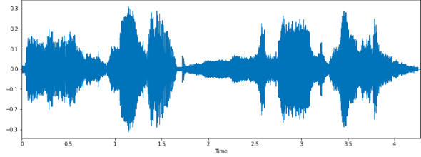
4. Waveform visualization : To visualize the sampled signal and plot it, we need two Python libraries—Matplotlib and Librosa. The following code depicts the waveform visualization of the amplitude vs the time representation of the signal.

%matplotlib inline
import matplotlib.pyplot as plt
import librosa.display

plt.figure(figsize=(14, 5))
#plotting the sampled signal
librosa.display.waveplot(x, sr=sr)

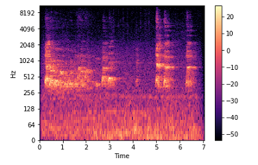
5. Spectrogram : A spectrogram is a visual representation of the spectrum of frequencies of a signal as it varies with time. They are time-frequency portraits of signals. Using a spectrogram, we can see how energy levels (dB) vary over time.

#x: numpy array
X = librosa.stft(x)
#converting into energy levels(dB)
Xdb = librosa.amplitude_to_db(abs(X))

plt.figure(figsize=(20, 5))
librosa.display.specshow(Xdb, sr=sr, x_axis='time', y_axis='hz')
plt.colorbar()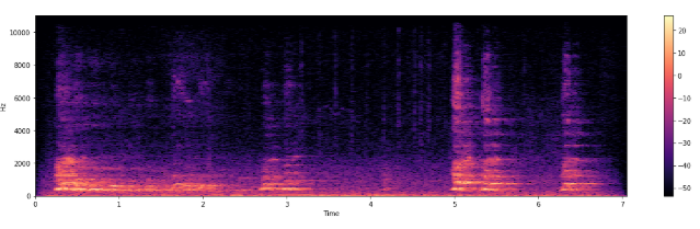

6. Log-frequency axis: Features can be obtained from a spectrogram by converting the linear frequency axis, as shown above, into a logarithmic axis. The resulting representation is also called a log-frequency spectrogram. The code we need to write here is:

librosa.display.specshow(Xdb, sr=sr, x_axis=’time’, y_axis=’log’)

Creating an audio signal and saving it

A digitized audio signal is a NumPy array with a specified frequency and sample rate. The analog wave format of the audio signal represents a function (i.e. sine, cosine etc). We need to save the composed audio signal generated from the NumPy array. This kind of audio creation could be used in applications that require voice-to-text translation in audio-enabled bots or search engines.

sr = 22050 # sample rate
T = 5.0    # seconds
t = np.linspace(0, T, int(T*sr), endpoint=False) # time variable
x = 0.5*np.sin(2*np.pi*220*t)# pure sine wave at 220 Hz

#playing generated audio
ipd.Audio(x, rate=sr) # load a NumPy array

librosa.output.write_wav('generated.wav', x, sr) # writing wave file in .wav format

So far, so good. Easy and fun to learn. But data pre-processing steps can be difficult and memory-consuming, as we’ll often have to deal with audio signals that are longer than 1 second. Compared to the images or number of pixels in each training item in popular datasets such as MNIST or CIFAR, the number of data points in digital audio is much higher. This may lead to memory issues.

Pre-processing of audio signals

Normalization

A technique used to adjust the volume of audio files to a standard set level; if this isn’t done, the volume can differ greatly from word to word, and the file can end up unable to be processed clearly.

#min = minimum value for each row of the vector signal
#max = maximum value for each row of the vector signal
def normalize(x, axis=0):
    return sklearn.preprocessing.minmax_scale(x, axis=axis)

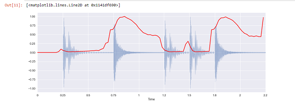
#Plotting the Spectral Centroid along the waveform
librosa.display.waveplot(x, sr=sr, alpha=0.4)
plt.plot(t, normalize(spectral_centroids), color='r')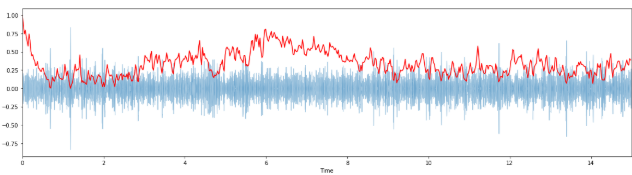

Pre-emphasis

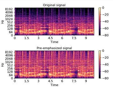
Pre-emphasis is done before starting with feature extraction. We do this by boosting only the signal’s high-frequency components, while leaving the low-frequency components in their original states. This is done in order to compensate the high-frequency section, which is suppressed naturally when humans make sounds.

import matplotlib.pyplot as plt
y, sr = librosa.load(audio_file.wav, offset=30, duration=10)
y_filt = librosa.effects.preemphasis(y)
# and plot the results for comparison
S_orig = librosa.amplitude_to_db(np.abs(librosa.stft(y)), ref=np.max)
S_preemph = librosa.amplitude_to_db(np.abs(librosa.stft(y_filt)), ref=np.max)

librosa.display.specshow(S_orig, y_axis='log', x_axis='time')
plt.title('Original signal')
librosa.display.specshow(S_preemph, y_axis='log', x_axis='time')
plt.title('Pre-emphasized signal')

Feature extraction from audio signals

Up until now, we’ve gone through the basic overview of audio signals and how they can be visualized in Python. To take us one step closer to model building, let’s look at the various ways to extract feature from this data.

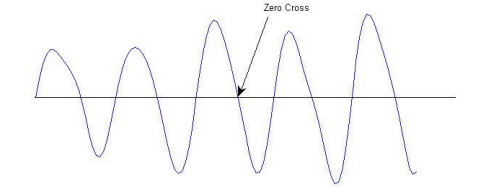
Zero Crossing Rate

The number times over a given interval that the signal’s amplitude crosses a value of zero. Essentially, it denotes the number of times the signal changes sign from positive to negative in the given time period. If the count of zero crossings is higher for a given signal, the signal is said to change rapidly, which implies that the signal contains the high-frequency information, and vice-versa.

#zero crossings to be found between a given time
n0 = 9000
n1 = 9100
plt.figure(figsize=(20, 5))
plt.plot(x[n0:n1])
plt.grid()

zero_crossings = librosa.zero_crossings(x[n0:n1], pad=False)
zero_crossings.shape

Spectral Rolloff

The rolloff frequency is defined as the frequency under which the cutoff of the total energy of the spectrum is contained, eg. 85%. It can be used to distinguish between harmonic and noisy sounds.

y, sr = librosa.load(librosa.util.example_audio_file())
# Approximate maximum frequencies with roll_percent=0.85 (default)
rolloff = librosa.feature.spectral_rolloff(y=y, sr=sr)

# Approximate minimum frequencies with roll_percent=0.1
rolloff = librosa.feature.spectral_rolloff(y=y, sr=sr, roll_percent=0.1)

MFCC

One popular audio feature extraction method is the Mel-frequency cepstral coefficients (MFCC), which has 39 features. The feature count is small enough to force the model to learn the information of the audio. 12 parameters are related to the amplitude of frequencies. The extraction flow of MFCC features is depicted below:

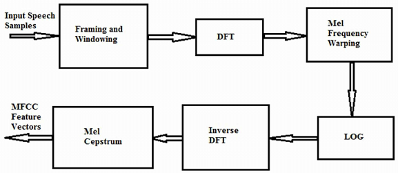
Framing and Windowing: The continuous speech signal is blocked into frames of N samples, with adjacent frames being separated by M. The result after this step is called spectrum.
Mel Frequency Wrapping: For each tone with a frequency f, a pitch is measured on the Mel scale. This scale uses a linear spacing for frequencies below 1000Hz and transforms frequencies above 1000Hz by using a logarithmic function.
Cepstrum: Converting of log-mel scale back to time. This provides a good representation of a signal’s local spectral properties, with the result as MFCC features.

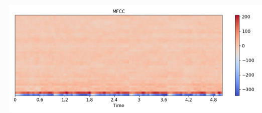
The MFCC features can be extracted using the Librosa Python library we installed earlier:

librosa.feature.mfcc(x, sr=sr)

Where x = time domain NumPy series and sr = sampling rate

Chroma Frequencies

The entire spectrum is projected onto 12 bins representing the 12 distinct semitones (or chroma) of the musical octave. The human perception of pitch is periodic in the sense that two pitches are perceived as similar if they differ by one or several octaves (where 1 octave=12 pitches).

x, sr = librosa.load('audio.wav')
ipd.Audio(x, rate=sr)

hop_length = 512
# returns normalized energy for each chroma bin at each frame.
chromagram = librosa.feature.chroma_stft(x, sr=sr, hop_length=hop_length)
plt.figure(figsize=(15, 5))
librosa.display.specshow(chromagram, x_axis='time', y_axis='chroma', hop_length=hop_length, cmap='coolwarm')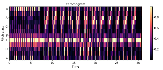

Conclusion

In this article on how to work with audio signals in Python, we covered the following sub-topics:

Loading and visualizing audio signals
Techniques of pre-processing of audio data by pre-emphasis, normalization
Feature extraction from audio files by Zero Crossing Rate, MFCC, and Chroma frequencies

Thanks for sticking till the end!