Understanding the Mathematics behind Support Vector Machines

In this post, we’re going to unravel the mathematics behind a very famous, robust, and versatile machine learning algorithm: support vector machines. We’ll also gain insight on relevant terms like kernel tricks, support vectors, cost functions for SVM, etc.

What is a support vector machine?

A support vector machine (SVM) is a supervised machine learning algorithm that can be used for both classification and regression tasks. In SVM, we plot data points as points in an n-dimensional space (n being the number of features you have) with the value of each feature being the value of a particular coordinate.

The classification into respective categories is done by finding the optimal hyperplane that differentiates the two classes in the best possible manner.

Hyperplanes

Hyperplanes can be considered decision boundaries that classify data points into their respective classes in a multi-dimensional space. Data points falling on either side of the hyperplane can be attributed to different classes.

A hyperplane is a generalization of a plane:

in two dimensions, it’s a line.
in three dimensions, it’s a plane.
in more dimensions, you can call it a hyperplane.

Let’s consider a two-dimensional space. The two-dimensional linearly separable data can be separated by the equation of a line—with the data points lying on either sides representing the respective classes.

The function of the line is y=ax+by. Considering x and y as features and naming them as x1,x2….xn, it can be re-written as:

If we define x = (x1, x2) and w = (a, −1), we get:

This equation is derived from two-dimensional vectors. But in fact, it also works for any number of dimensions. This is the equation for a hyperplane:

Finding the best hyperplane

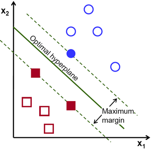
By looking at the data points and the resultant hyperplane, we can make the following observations:

Hyperplanes close to data points have smaller margins.
The farther a hyperplane is from a data point, the larger its margin will be.

This means that the optimal hyperplane will be the one with the biggest margin, because a larger margin ensures that slight deviations in the data points should not affect the outcome of the model.

For linear data:

For non-linear data:

What is a large margin classifier?

SVM is known as a large margin classifier. The distance between the line and the closest data points is referred to as the margin. The best or optimal line that can separate the two classes is the line that has the largest margin. This is called the large-margin hyperplane.

The margin is calculated as the perpendicular distance from the line to only the closest points.

What are support vectors?

Since the margin is calculated by taking into account only specific data points, support vectors are data points that are closer to the hyperplane and influence the position and orientation of the hyperplane.

Using these support vectors, we maximize the margin of the classifier. Deleting the support vectors will change the position of the hyperplane. These are the points that help us build our SVM.

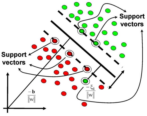
Basically, support vectors are imaginary or real data points that are considered landmark points to determine the shape and orientation of the margin.

The objective of the SVM is to find the optimal separating hyperplane that maximizes the margin of the training data.

The SVM Classifier

The hypothesis function h is defined as:

The point above or on the hyperplane will be classified as class +1, and the point below the hyperplane will be classified as class -1.

Computing the (soft-margin) SVM classifier amounts to minimizing an expression of the form

We focus on the soft-margin classifier since choosing a sufficiently small value for lambda yields the hard-margin classifier for linearly-classifiable input data.

Implementing SVM in Python with sklearn

It merely takes four lines to apply the algorithm in Python with sklearn: import the classifier, create an instance, fit the data on the training set, and predict outcomes for the test set:

Tuning parameters according to the task at hand

Setting C: C is 1 by default, and it’s a reasonable default choice. If you have a lot of noisy observations, you should decrease the value of C. It corresponds to the regularization of the hyperplane; or put another way, it smooths the curve of the hyperplane.

2. Setting gamma: If low, then the points far away from the hyperplane will also be considered for hyperplane tuning.

Kernel trick

In SVMs, there can be a lot of new dimensions, each of them possibly involving a complicated calculation. Doing this for every vector in the dataset can be a lot of work. Here’s a trick: SVM doesn’t need the actual vectors to work its magic—it actually can get by with only the dot products between them.

Imagine the new space we want is:

We need to figure out what the dot product in that space looks like:

a · b = xa · xb + ya · yb + za · zb
a · b = xa · xb + ya · yb + (xa² + ya²) · (xb² + yb²)

Now, tell the SVM classifier to do its thing, but using the new dot product — we call this a kernel function.

The scikit-learn library in Python provides us a lot of options to choose as our kernel, and we can design our own custom kernels too. You can learn more about kernel functions here.

This is called the Kernel Trick. Normally, the kernel is linear, and we get a linear classifier. However, by using a nonlinear kernel as mentioned in the scikit-learn library, we can get a nonlinear classifier without transforming the data or doing heavy computations at all.

Advantages of SVM

It’s very effective in high-dimensional spaces as compared to algorithms such as k-nearest neighbors.
It’s still effective in cases where the number of dimensions is greater than the number of samples.
SVM is versatile: different kernel functions can be specified for the decision function. Common kernels are provided, but it’s also possible to specify custom kernels.
It works really well with a clear margin of separation.

Disadvantages of SVM

The main disadvantage of SVM is that it has several key parameters like C, kernel function, and Gamma that all need to be set correctly to achieve the best classification results for any given problem. The same set of parameters will not work optimally for all use cases.
SVMs do not directly provide probability estimates—these are calculated using an expensive five-fold cross-validation process (see scores and probabilities, below).
It doesn’t perform very well when the dataset has more noise, i.e. target classes are overlapping.

How to prepare your data for SVM?

Numerical Inputs: SVM assumes that your inputs are numeric. If you have categorical inputs, you may need to covert them to binary dummy variables (one variable for each category).
SVM is not scale invariant, so it’s highly recommended to scale your data. For example, scale each attribute on the input vector X to [0,1] or [-1,+1], or standardize it to have mean 0 and variance 1.

Conclusion

In this post, we read about support vector machines (SVMs) in detail and gained insights about the mathematics behind it. Despite being widely used and strongly supported, it has its share of advantages and disadvantages.

Let me know if you liked the article and how I can improve it. All feedback is welcome. I’ll be exploring the mathematics involved in other foundational machine learning algorithms in future posts, so stay tuned.