Understanding the Mathematics Behind Naive Bayes

In this post, we’re going to dive deep into one of the most popular and simple machine learning classification algorithms—the Naive Bayes algorithm, which is based on the Bayes Theorem for calculating probabilities and conditional probabilities.

Before we jump into the Naive Bayes classifier/algorithm, we need to know the fundamentals of Bayes Theorem, on which it’s based.

Bayes Theorem

Given a feature vector X=(x1,x2,…,xn) and a class variable Ck, Bayes Theorem states that:

P(Ck|X)=P(X|Ck)P(Ck)/(P(X)), for k=1,2,…,K

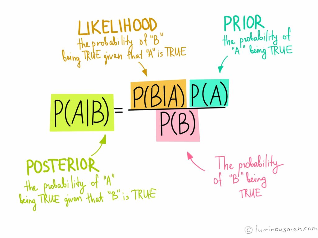
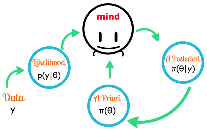
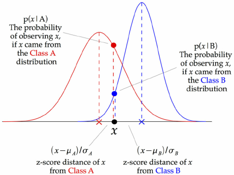
We call P(Ck∣X) the posterior probability, P(X∣Ck) the likelihood, P(Ck) the prior probability of a class, and P(X) the prior probability of the predictor. We’re interested in calculating the posterior probability from the likelihood and prior probabilities.

Using the chain rule, the likelihood P(X∣Ck) can be decomposed as:

The term “Naive” and feature independence

It’s quite tedious to calculate the set of probabilities for all values again and again. Fortunately, with the naive conditional independence assumption, the conditional probabilities are independent of each other.

In terms of machine learning, we mean to say that the features provided to us are independent and do not affect each other, and this does not happen in real life. The features depend on the occurrence or value of another, which is simply ignored by the Naive Bayes classifier and is hence given the term, “NAIVE”.

Thus, by conditional independence, we have:

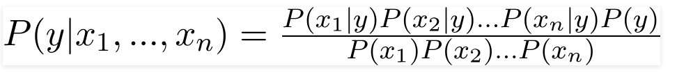
And the posterior probability can then be written as:

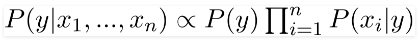
since the denominator remains constant for all values.

Naive Bayes Classifier

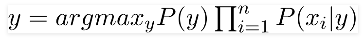
The discussion so far has derived the independent feature model—that is, the naive Bayes probability model. The Naive Bayes classifier combines this model with a decision rule. One common rule is to pick the hypothesis that’s most probable; this is known as the maximum a posteriori or MAP decision rule. The corresponding classifier, a Bayes classifier, is the function that assigns a class label for some k as follows:

Types of Naive Bayes Classifiers

Gaussian: Used in classification, and it assumes that features follow a normal distribution.

Multinomial: Used for discrete counts. For example, let’s say we have a text classification problem. Here we can consider Bernoulli trials, which are one step further, and instead of counting the instances of a “word occurring in the document”, we have a “count how often a word occurs in the document”. Broadly, you can think of it as the “number of times outcome number x_i is observed over the n trials”.
Bernoulli: The binomial model is useful if your feature vectors are binary (i.e. zeros and ones). One application would be text classification with a ‘bag of words’ model, where the 1s & 0s are counts of “word occurs in the document” and “word does not occur in the document” respectively.

Naive Bayes in Python with sklearn

It merely takes four lines to apply the algorithm in Python with sklearn: import the classifier, create an instance, fit the data on training set, and predict outcomes for the test set:

How to prepare your data for Naive Bayes

Categorical Inputs: Naive Bayes assumes label attributes such as binary, categorical, or nominal.
Log Probabilities: The calculation of the likelihood of different class values involves multiplying a lot of small probabilities together, which can result in an underflow of values, or computationally very low values. As such, it’s good practice to use a log transform of the probabilities to avoid this underflow.
Kernel Functions: Instead of assuming a Gaussian distribution for numerical input values, which usually fits all kinds of numerical values, complex distributions can be used.
Gaussian Inputs: If the input variables are real-valued, a Gaussian distribution is assumed. In this case, the algorithm will perform better if the univariate distributions of your data are Gaussian or near-Gaussian. This may require removing outliers.
Update Probabilities: When new data becomes available, you can simply update the probabilities of your model.

Advantages of Naive Bayes

When the assumption of independent predictors holds true, a Naive Bayes classifier performs better as compared to other models. If the Naive Bayes conditional independence assumption holds, then it will converge quicker than discriminative models like logistic regression.
Naive Bayes requires a small amount of training data to estimate the test data. So the training period takes less time.
Very simple, easy to implement, and fast. It can make probabilistic predictions.
It is highly scalable. It scales linearly with the number of predictor features and data points.
Can be used for both binary and multi-class classification problems.
Handles continuous and discrete data and is not sensitive to irrelevant features.

Disadvantages of Naive Bayes

The main limitation of Naive Bayes is the assumption of independent predictor features. Naive Bayes implicitly assumes that all the attributes are mutually independent. In real life, it’s almost impossible that we get a set of predictors that are completely independent or one another.
If a categorical variable has a category in the test dataset, which was not observed in training dataset, then the model will assign a 0 (zero) probability and will be unable to make a prediction. This is often known as Zero Frequency. To solve this, we can use a smoothing technique. Details on additive smoothing or laplace smoothing can be found here.

Sources for getting started with Naive Bayes

Here are a few resources for you to experiments with that apply Naive Bayes to publicly-available repositories:

Conclusion

In this post, we read about the Naive Bayes classifier in detail, and gained insights about the mathematics and assumptions behind it. Despite being widely used and strongly supported, it has it’s share of advantages and disadvantages.

Let me know if you liked the article. All feedback is welcome. Stay tuned, as I’ll be writing more about the math involved with other machine learning algorithms, as well.