
Python-PyTorch

Loss functions are among the most important parts of neural network design. A loss function helps us interact with a model, tell it what we want — this is why we classify them as “objective functions”. Let us look at the precise definition of a loss function.
In deep learning, an objective function is one whose output has to be minimized. Thus, the optimization algorithm needs to find a minima from the objective function. This is usually done by a backpropagation algorithm that calculates the gradients and then passes them over to the optimization algorithm. The optimization algorithm then changes the neural network parameters and weights so as to arrive at a lower objective function output.
It should be noted that the goal of the optimization algorithm isn’t always minimizing the objective function. There are times when the objective function must be maximized. When we’re minimizing it, we also call it the cost function, loss function, or error function.
Thus, it’s plainly evident that the loss function is of primary importance, and without the loss function, we cannot make the model understand what we need it to achieve.
There are two types of losses —
A) Regression loss — Regression loss functions in deep learning are functions or models that predict a quantity, and are applied to regression models. Examples of regression loss include the mean squared error loss (L2 loss) and the mean absolute error loss (L1 loss)
B) Classification loss — Classification functions or models classify the input to one of the classes served to it, instead of predicting a value or quantity. These loss functions help these models perform more effective classification.
While I’ll cover regression briefly below, I’ll focus the majority of this article on classification loss, as more models in deep learning are devoted to classification tasks. If you would like an article specifically on regression loss, let me know in the comments 😉
Regression Loss
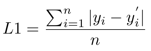
L1 Loss
L1 loss, also known as mean absolute error (MAE) is, as the name suggests, the mean of the absolute losses over all the variables. Thus, we can write MAE as:
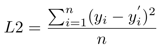
L2 Loss
L2 loss is also known as mean squared error (MSE). L2 loss, as one can easily infer, is the mean of the squared differences between the predicted variable and the label variable. It is expressed as:
Both L1 and L2 loss can be easily imported from the PyTorch library in Python. They can also be easily implemented using simple calculation-based functions. Here’s a code snippet for the PyTorch-based usage:
Try making your own function definitions for these loss functions, as they’re quite simple and would be easy to begin with.
Classification Loss
Now that we’ve briefly explored the simple loss functions for regression models, we’ll move on to classification loss functions. An activation function is generally required at the output layer so that the output gets formatted in a way that’s easier for the loss function to process.
An activation function is one that gives the model a non-linear aspect. Without activations, we would have simple linear models that would be limited in what they could learn. With the help of activation functions, we can make neural networks learn more by introducing forms of non-linearity.
It should be noted that an activation function helps the loss function “recognize” the output. In all likelihood, the loss function will not work without the same or similar activation function. Before diving into the loss functions, let us explore some output activation functions.
Sigmoid
The sigmoid activation layer is a layer that squashes the input it takes into a value in the range (0,1). This is necessary for converting the output into a probability. The sigmoid curve is a characteristic ‘S’ shaped curve.
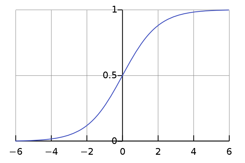
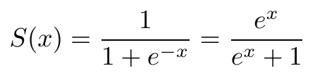
The equation that generates the curve is:
Softmax
Softmax is an activation function that computes the normalized exponential function of all the units in the layer. Mathematically, it can be expressed as:
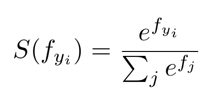
Looks tricky, eh? Let me break it down for you. What a softmax activation function does is take an input vector of size N, and then adjusts the values in such a way that each value is in between zero and one. Moreover, the sum of the N values of the vector sum up to 1, as a normalization of the exponential.
In order to use the softmax activation function, our label should be one-hot-encoded. The value of N here corresponds to the number of classes we need the model to work on.
Tanh
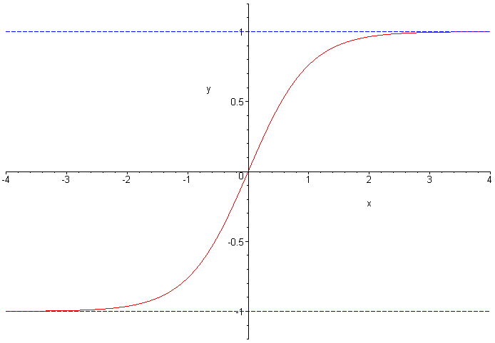
The tanh activation function is very similar to the sigmoid function with respect to its shape. It computes just the hyperbolic tangent of the input—as a result of which, the input gets squashed in the range of (-1,1). The curve can be visualized as follows:
So now that we know about various output activations, let’s move on to the loss functions.
NLL Loss
NLL stands for Negative Log Likelihood. It’s used only in models that have softmax as an output activation layer. Mathematically, we can write NLL loss as:
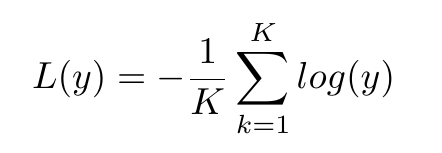
Simple as that? Yep! But how does simply minimizing this loss function help us arrive at a better solution? The negative log likelihood is derived from the estimation of maximum likelihood. In other words, we attempt to maximize the log likelihood of the model, and thus minimize the NLL.
An important point to note is that maximizing the log of the probability function works similarly to maximizing the probability function, as the logarithm is a monotonically increasing curve. This ensures that the maximum value of the log of the probability occurs at the same point as the original probability function.
Let’s see a short PyTorch implementation of NLL loss:
import torch
from torch import nn
loss=nn.NLLLoss()
data=torch.randn(5,16,10,5)
conv=nn.Conv2d(16,4,(3,3))
m=nn.LogSoftmax(dim=1)
target=torch.empty(5,8,8,dtype=torch.long).random_(0,4)
output=loss(m(conv(data)),target)
output.backward()
Cross-Entropy Loss
A neural network is expected, in most situations, to predict a function from training data and, based on that prediction, classify test data. Thus, networks make estimates on probability distributions that have to be checked and evaluated. Cross-entropy is a function that gives us a measure of the difference between two probability distributions for a given random variable or set of events.
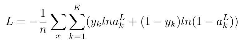
Categorical cross-entropy works on sigmoid activation. Mathematically, it can be expressed as follows:
One primary point of confusion people have is that the negative log likelihood and cross-entropy are very similar cost functions. What makes them different? Here’s an explanation to dispel that confusion.
Cross-entropy and negative log likelihood are essentially the same cost function—i.e. they both serve to maximize the log likelihood. However, the output of a sigmoid activation function cannot be directly applied to a NLL loss function — it has to be applied to a cross-entropy function. Similarly, the NLL loss function can take the output of a softmax layer, which is something a cross-entropy function cannot do!
The cross-entropy function has several variants, with binary cross-entropy being the most popular. BCE loss is similar to cross-entropy but only for binary classification models—i.e. models that have only 2 classes.
Let’s see a PyTorch implementation of cross-entropy loss —
import torch
from torch import nn
loss = nn.CrossEntropyLoss()
input = torch.randn(6, 9, requires_grad=True)
sigmoid=nn.Sigmod()
out=sigmoid(input)
target = torch.empty(6, dtype=torch.long).random_(5)
output = loss(out, target)
output.backward()
What’s Next?
Try to develop your own code for these loss functions — it will help you get the hang of them, and when the time comes, you’ll be able to identify the loss function necessary for dealing with a specific problem. Let me know in the comments if I can help in any way;)
Check out my blog for faster updates and subscribe for quality content 😀
Hmrishav Bandyopadhyay is a 2nd year Undergraduate at the Electronics and Telecommunication department of Jadavpur University, India. His interests lie in Deep Learning, Computer Vision, and Image Processing. He can be reached at — hmrishavbandyopadhyay@gmail.com || https://hmrishavbandy.github.io
Comments 0 Responses