
Following what we learned about human vision, we’re now going to transfer some of that knowledge to computer vision (exciting right?!).
Very quickly, to quickly explain/recap this series, Joseph Redmon released a set of 20 lectures on computer vision in September 2018. As he’s an expert in the field, I wrote a lot of notes while going through his lectures. I am tidying my notes for my own future reference but am posting them on Medium also, to hopefully be useful for others.
Table of contents
What is an image?
To start moving on from human vision, let’s start with the very fundamental question: “What is an image?”
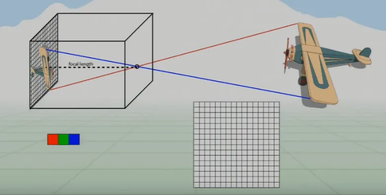
Our eyes project light onto our retinas flipped through a single point where the focal length is the distance to the “virtual” image. Essentially, it’s a projection of the 3D world onto a 2D plane.
Lets continue this idea and imagine the retina as a 2D grid of RGB color sensors upon which an image is projected.
We also know that we have red, blue, and green cones in our eyes to detect different amounts of these three colors (which combine to every visible color). Therefore, the grid needs an RGB filter with twice as many green filters as the others, as we respond to green the most (we judge brightness using our green sensors).
The filter we use is called a Bayer Pattern Filter and goes over the sensors to only allow certain light to reach certain sensors:
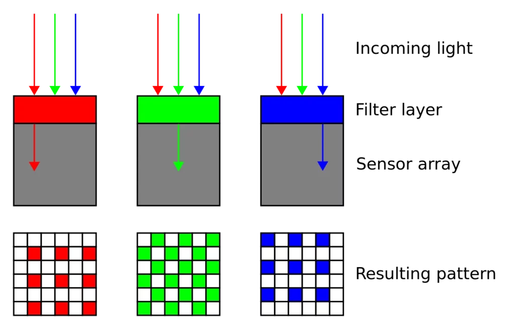
As you can see above, only red light gets through the red filter, green through the green filter and blue through the blue filter. Layering this onto our 2D grid of sensors, we get a pattern like this:
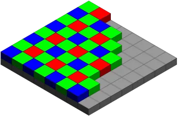
You can see there are twice as many green filters as the other two, and they’re arranged over the sensors to create a matrix of light in which each value represents a sensor reading that’s commonly called a pixel value.
These values are of course bounded below at 0 but also bounded above as the sensors in our eyes get saturated. This upper bound is usually 255 so that each pixel can fit into a byte and still represent more colors than humans can even distinguish between (around 1 million). The higher the value, the higher the amount of light that hit that pixel.
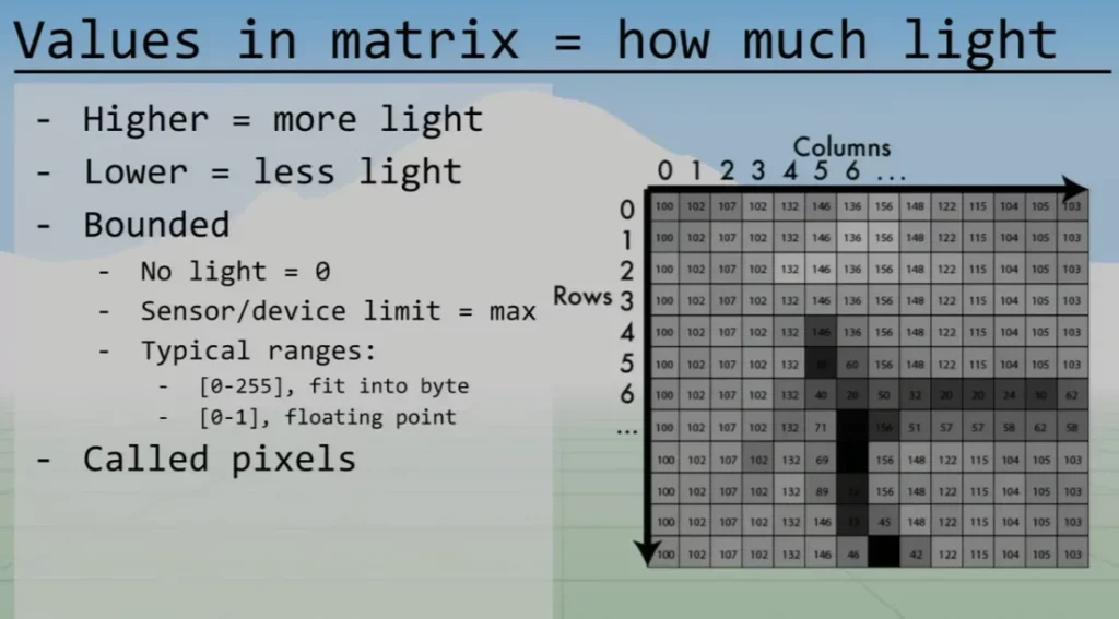
To identify one pixel in this matrix you can use row, column (r, c) (like in mathematics) or x, y coordinates, which tends to be used in computer vision. Both of these notations consider the upper-left pixel the origin (0, 0), and which one you use doesn’t really matter as long as you’re consistent. This is very useful to know however if you’re reading StackOverflow, etc…
So this is how a camera captures an image in a human (influenced) manner, but how is this matrix then stored for our uses?
Storing an Image: 3D Tensors with RGB Channels
If we take the above matrix and split it into three grids, each representing an RGB channel, we have a matrix of values of each color at each pixel. The red matrix, for example, is full of values representing how much red hit each sensor.
If we extend the coordinate system to (x, y, c), where c represents the color channel, our color image is now represented by a 3D tensor.
In the RGB color space, “c” can be 0, 1, or 2, where 0 is red, 1 is green, and 2 is the blue matrix. Let’s visualize this to avoid confusion:
Once this tensor is filled with values, these channels can be combined to recreate images, as discussed in my human vision article.
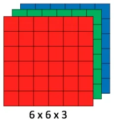
To extend this into a usual image size: 1920 x 1080 x 3 is 1920px wide, 1080px tall, and has 3 channels.
To actually store this in memory, however, we store it as a 1D vector (120, 127, 56, …). This is almost always row major but MATLAB has to be different and use column major mapping (oh, the pain from my math undergrad days).
Row major is often called HW (height width) and column major is WH (width height). Basically, the right most letter is the “closest together”, which I realize isn’t immediately intuitive, so here’s one of Joseph Redmon’s slides followed by a simple example I’ve constructed:
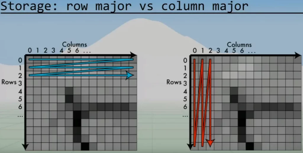
So, row major is HW and blue in the above slide. Column major is therefore WH and red. Given the following 3×3 grid, let’s explain this “closer together” remark.
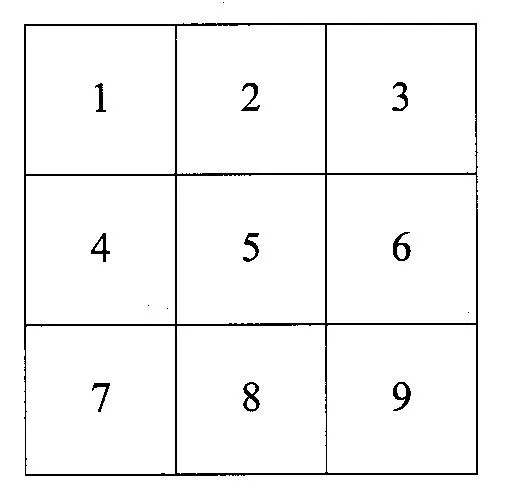
If you travel the width (rightmost letter in HW) the values in the vector are close together, e.g. going along the top row in bold (1, 2, 3, 4, 5, 6, 7, 8, 9).
If you travel the height however, the values are further apart and you jump along the vector. e.g. going down the first column in bold (1, 2, 3, 4, 5, 6, 7, 8, 9).
Conversely:
If you travel the height (right most letter in WH) the values in the vector are close together e.g. going down the first column in bold (1, 4, 7, 2, 5, 8, 3, 6, 9).
If you travel the width however, the values are further apart and you jump along the vector. e.g. going along the first row in bold (1, 4, 7, 2, 5, 8, 3, 6, 9).
Now let’s add channels…You sometimes see HWC in which the channels are interleaved:
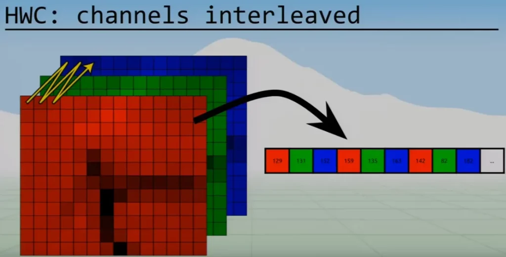
Again, with these three letter acronyms, as you travel along the rightmost letter, you’ll jump shorter distances through the output vector. This extends so that as you travel through the leftmost letter, you jump much further through the vector.
You can see in the HWC example above that you pop along the vector to get the next channel value, but you’d have to jump a huge distance to find the first value in the second row of the red channel.
We’ll use the CHW the most, which basically stacks each channel on top of each other, and then is row major (all red row major, then all green, and then all blue).
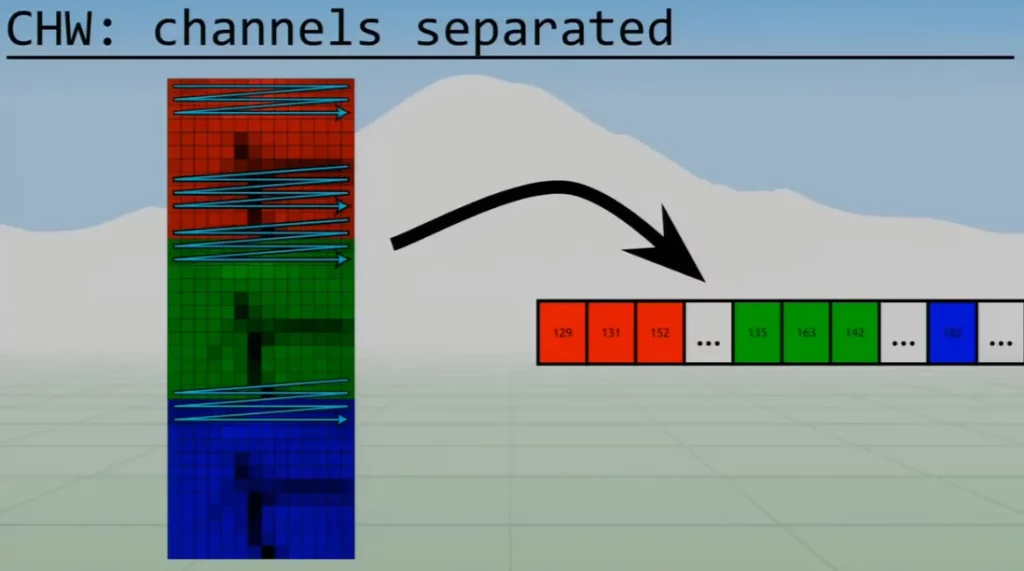
CHW is what most libraries use, hence why we’ll use it throughout these articles.
Are we done now? Can we represent an image in a 1D vector? Yes, but only for RGB images. So what about other color spaces?
Storing an Image: Other Color Spaces
To make image manipulation easier, we commonly convert images from the RGB color space to HSV or Hue, Saturation, Value.
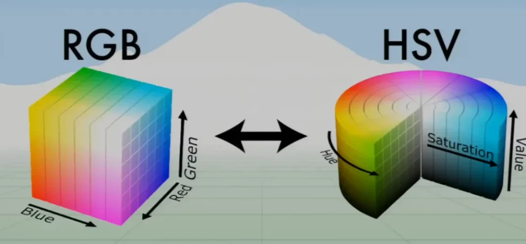
In RGB, the color is tied with its luminescence, whereas in HSV they’re separated, which allows us to manipulate an image in a much more straightforward manner. We’ll cover some examples of this later.
This conversion is very difficult to explain in text, but the diagram below illustrates it well:
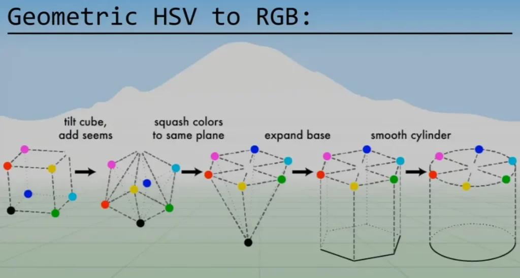
This RGB cube (in figure 10) is tilted and squashed so that all the colors are on the same plane. The black point is then expanded to create the base of the HSV cylinder shown in figure 10.
Every image in the HSV color space is still represented by a 3D tensor with three channels. The difference is that the channels are no longer red, green, and blue (RGB) but instead hue, saturation, and value (HSV).
As we’ve expanded the black point into the base of the cylinder, it’s completely black, and the color is then most vibrant at the top of the cylinder. This is the value in HSV. Hue represents which color the pixel is, and the central column of this is white. This means that the closer a point is to the central core of the cylinder, the whiter it is (or less saturated).
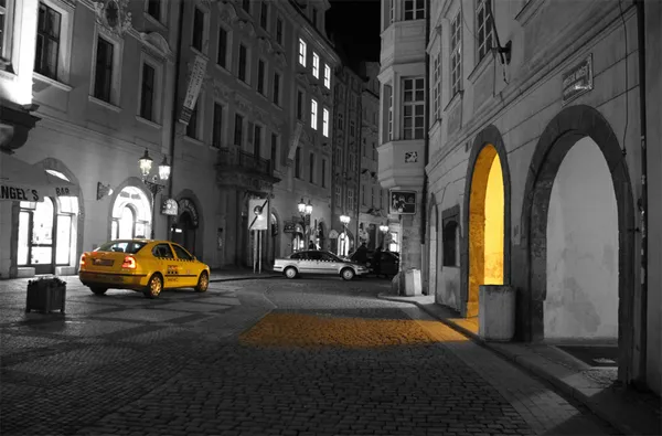
We can see this in the following example:
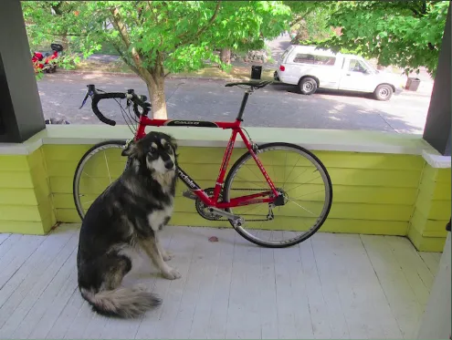
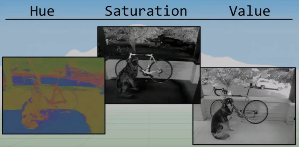
You can see that the hue still shows the yellow wall and red bike from the original image, but the floor looks blue, even though it’s grey in the original image.
This is because even though the hue is blue, the saturation is very low. In the saturation image, you can see that the wall and bike are very bright, which tells us that the yellow and red in the hue image look that color. The floor, however, has a low saturation and is therefore grey.
The value image looks grayscale but isn’t actually, as grayscale images are a lot more complicated than you’d initially think. As we know, green matters a lot more than red and blue in how we see the world, but this information is lost in value images and is therefore less accurate at representing our perception. The value image is just in black and white and represents how luminescent a pixel is.
In this color space, we can perform image manipulations that are much more difficult to perform if the image was represented in the RGB color space. For example, we could double all saturation values to over saturate the image.
and pointed out that this is a very common trick used to sell houses.
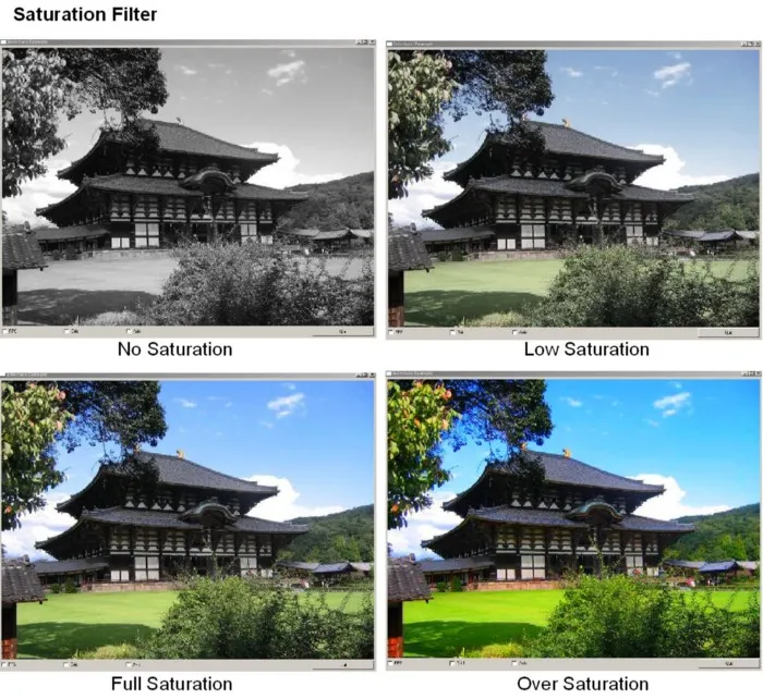
To reiterate, this is quite difficult to do in the RGB color space but very easy in HSV.
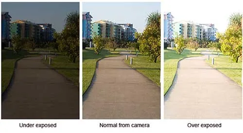
Similarly, we can very easily manipulate the exposure of an image by modifying its value (again, exposure is covered in part 1).
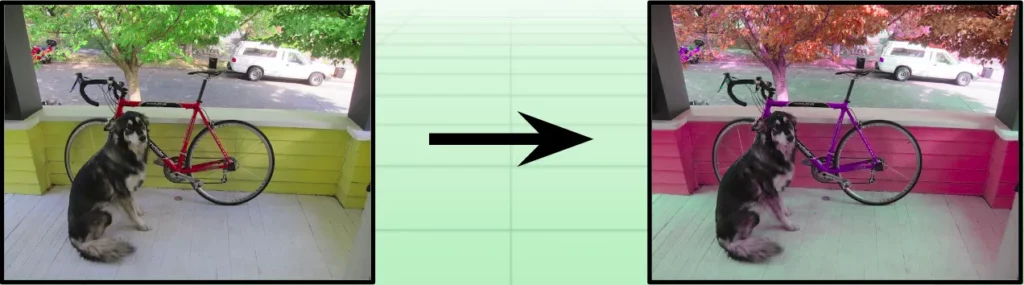
Changing the hue values changes the colors in the picture. This is often used in Photoshop to tweak colors of objects in photos; but is has another very interesting use.
Machine learning, especially deep learning, requires a lot of data to train. To complicate matters, this data needs to be annotated, which is difficult to collect at scale. By manipulating the hue of an already annotated image, you can generate more labeled data to train models. These images look very similar to us but don’t to computers, so this can be used to significantly increase the size of a dataset.
These examples are fairly simple, but you can also perform more complicated manipulations easily. For example, you could replace the hue matrix with a pattern to get psychedelic results or add threshholding to an image’s saturation matrix to desaturate all colors apart from one to get some cool results like this:
These manipulations are all used very practically every day for things like Instagram filters and branding. Another image manipulation we use all the time is image resizing. Whether viewing images on different screens or pinching your phone screen to zoom, this is done in different ways depending on the use case.
Image Interpolation and Resizing
So we have these tensors that represent images by mapping integers to pixel values. What if we wanted to pass in real values to move smoothly across the image rows and columns?
We use interpolation to do exactly this.
An image is basically a bunch of discrete points at which we record amounts of light, so (0,0) is not the top left corner of an image but the top left point.
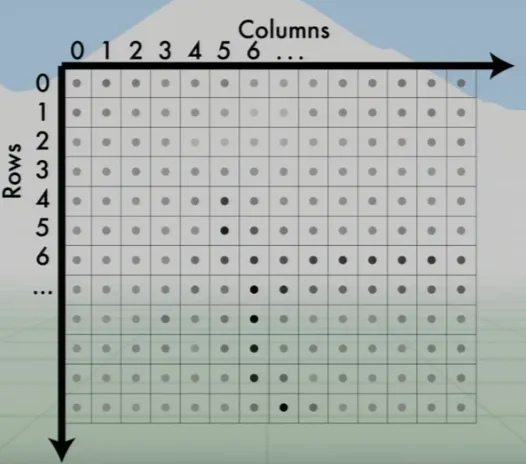
As (0,0) is this dot, and we don’t have any information between dots, all known information is a grid and not a real plane. If we reduced the number of these points, the image would become more pixelated, so to increase resolution we’d have to add points [the top point could be (0.25,0.25) for example].
We can do this using several methods.
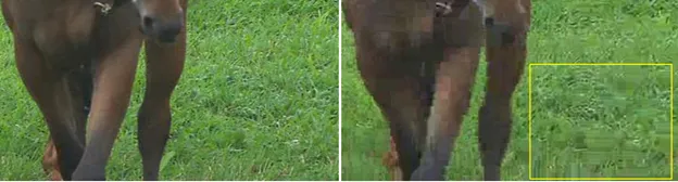
Nearest Neighbor
Given a real (x,y), the nearest neighbor method simply returns the closest point in the grid that we have info for.
As you can imagine, this just duplicates pixels and therefore looks blocky, but it’s very fast.
Triangle Interpolation
Sometimes data is less structured and more sparse, as sensors may break. In these cases, we can use triangle interpolation, which returns the weighted sum of the three nearest values to (x,y). As it returns the weighted sum, blue and green are still represented even if the nearest neighbors are mostly red.
This triangle interpolation tends to work better than the usual one point nearest neighbor method because of this weighted sum across multiple points. For this same reasoning, bilinear interpolation is popular.
Bilinear Interpolation
Given a real (x,y), we grab a box of four points around (x,y). Using these points, we calculate the weighted sum of their values (just like triangle).
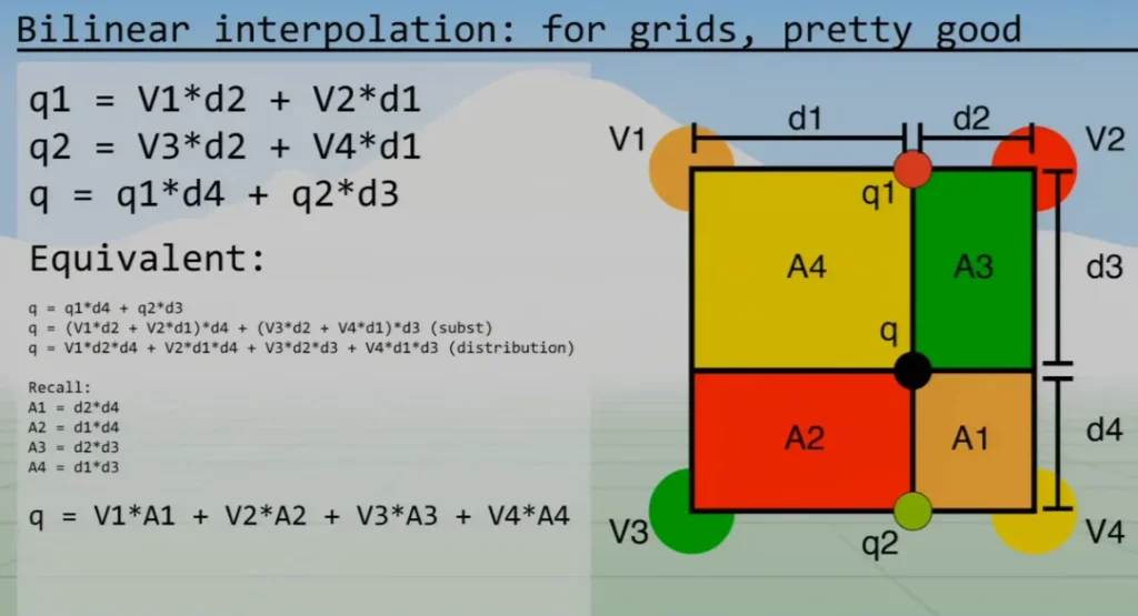
If you notice, the vertices are in the opposite corners of their corresponding areas. Therefore, if a point is really close to V4, the area A4 would be huge and weights the final value towards V4.
As you can see in figure 18, the value at real point (x,y) called q is calculated as follows:
This method is much smoother than the nearest neighbor method, but also far more complex. Nearest neighbor simply looks up one pixel value, whereas bilinear interpolation looks up four values and then performs some computation. The tradeoff between speed and quality needs to be considered when choosing a method.
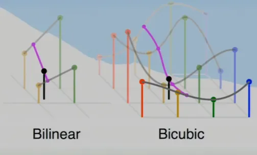
Bicubic Interpolation
The above bilinear interpolation is a linear interpolation of two linear interpolations.
Bicubic interpolation is a cubic interpolation of four cubic interpolations and therefore needs to look up sixteen pixel values and complete a lot more math. This is, of course, much slower, but it’s also a lot smoother than the other methods; so again, the balance depends on your use case.
In summary of how to resize an image, we:
- Map each pixel in the new desired image to old image coordinates.
- Interpolate using one of the methods described above.
- Assign the returned interpolation values in the new image.
This is the same whether we’re increasing the image resolution or shrinking it. Of course, in the latter we get a lot of artifacting.
Conclusion
We now know how images are represented and how computers store them in the two most common color spaces (RGB and HSV). We’ve covered some image manipulations (some useful for labeled data generation for deep learning) and dived into interpolation methods for resizing.
How an image is stored is very important to pay attention to, as problems can occur if you pass a tensor with the wrong encoding to a library, and this is a common pain point when starting out.
In the next article, we’ll cover some more advanced resizing techniques to avoid common problems, some filtering methods, and convolution.

Comments 0 Responses