
With recent developments in deep learning, neural networks are getting larger and larger. For example, in the ImageNet recognition challenge, the winning model, from 2012 to 2015, increased in size by 16 times. And in just one year, for Baidu’s Deep Speech model, the number of training operations increased by 10 times.
Generally speaking, deep learning in embedded systems has 3 main challenges:
- As model size becomes larger, it becomes more difficult for models to be deployed on mobile phones. If the model is over 100 MB, you cannot (generally speaking) download them until you can connect to Wi-Fi.
- Training speed becomes extremely slow. For example, the original ResNet152, which is less than 1% more accurate than ResNet101, takes 1.5 weeks to train on 4 distributed GPUs.
- Such bulky models also struggle with energy efficiency. For example, AlphaGo beating Lee Sedol in Go took 1,920 CPUs and 280 GPUs to train, which costs approximately $3,000 in terms of electricity.
In this context, running neural networks on resource-constrained devices requires joint solutions from data engineering and data science, which are sometimes called “algorithm and hardware co-design”. The figure below from Song Han class at Stanford, from her video lecture titled Efficient Methods and Hardware for Deep Learning, illustrates this idea:
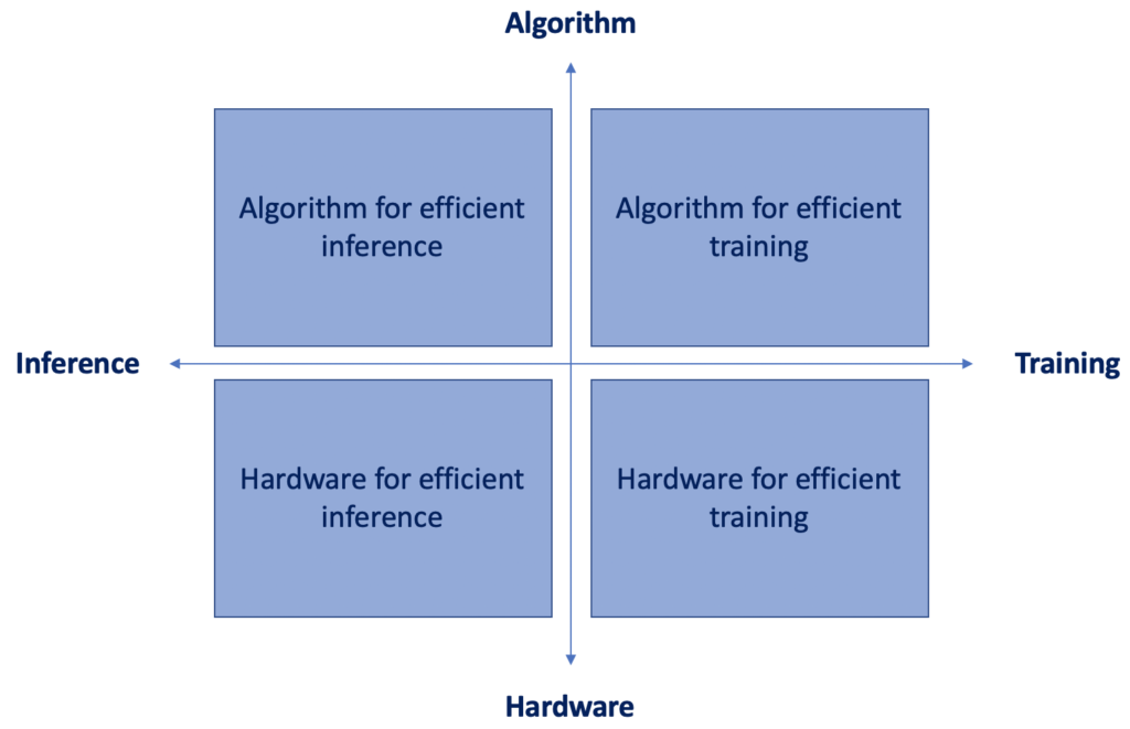
In this article, we’ll discuss the upper left part of the quadrant only. What are the state-of-the-art algorithms to do inference efficiently?
1 — Pruning Neural Networks
Contrary to what you may think, pruning has nothing to do with cutting trees! In machine learning, model pruning consists of removing unimportant weights in order to get a smaller and faster network.
Model pruning was first introduced in 1989 by Yann Le Cun in his paper “Optimal Brain Damage”. The idea is to take a fully trained network and prune weights whose deletion will cause the least increase in the objective function. The contribution of each parameter can be approximated using the Hessian matrix. Once unimportant weights have been removed, the smaller network can be trained once again, and the process can be repeated several times until the network has both a satisfying size and a reasonable performance.
Since then, plenty of pruning technique variations have been developed. In 2015, Han et al, in “Learning both Weights and Connections for Efficient Neural Networks”, introduced a three-step method that consists of training a neural network, then pruning connections whose weight is lower than a chosen threshold, and finally retraining the sparse network to learn the final weights for the remaining connections.
You may wonder: How is the pruning threshold determined? Good question! Both convolution and fully connected layers can be pruned; however, experience has shown that convolution layers are more sensitive to pruning than fully connected layers. Thus, the threshold is chosen according to the sensitivity of each layer, as shown in the figure below, which is taken from the research paper from Han et al.

According to the research paper, 173 hours were needed to retrain the pruned AlexNet on an NVIDIA Titan X GPU. But retraining time isn’t a key concern, because the end goal is to make the smaller model run quickly on a resource-constrained device.
On ImageNet, the method reduced the number of parameters of AlexNet by a factor of 9x (from 61 million parameters to 6.7 million) and of VGG-16 by a factor of 13x (from 138 million parameters to 10.3 million). After pruning, the storage requirements of AlexNet and VGGNet are much lower, and all weights can be stored on-chip rather than on off-chip DRAM (which takes significantly more energy to access).
2 — Deep Compression
Neural networks are both computationally intensive and memory intensive, making them difficult to deploy on embedded systems with limited hardware resources. To address this limitation, the Deep Compression paper from Han et al, introduced a 3-stage pipeline (shown below): pruning, trained quantization, and Huffman coding, which work together to reduce the storage requirements of neural networks by 35 to 49 times, without affecting their accuracy.

The method first prunes the network by learning only the important connections. Next, the method quantizes the weights to enforce weight sharing. Finally, the method uses Huffman coding. After the first two steps, the authors retrain the network to fine-tune the remaining connections and the quantized centroids. Pruning reduces the number of connections by 9 to 13 times. Quantization then reduces the number of bits that represent each connection from 32 to 5.
On ImageNet, the method reduced the storage required by AlexNet by 35 times (from 240 MB to 6.9 MB) without accuracy loss. The method also reduced the size of the VGG-16 pre-trained model by 49 times (from 552 MB to 11.3 MB), also without accuracy loss.
Finally, this deep compression algorithm facilitates the use of complex neural networks in mobile applications, where the application size and download bandwidth are constrained. When benchmarked on CPU, GPU, and mobile GPU, the compressed network has a 3 to 4 times layer-wise speedup and 3 to 7 times better energy efficiency.
3 — Data Quantization
In recent years, convolutional neural network-based methods have achieved great success in a large number of applications and have been among the most widely used architectures in computer vision. However, CNN-based methods are computational-intensive and resource-consuming, and thus are hard to be integrated into embedded systems such as smartphones, smart glasses, and robots. Field Programmable Gate Array (FGPA) is a promising platform for accelerating CNNs, but the limited bandwidth and on-chip memory size limit the performance of the FPGA accelerator for CNNs.
In the paper Going Deeper with Embedded FPGA Platform for CNN from researchers at Tsinghua University, a CNN accelerator design on embedded FPGA for ImageNet large-scale image classification was proposed. The authors empirically showed that inside the architecture of current state-of-the-art CNN models, the convolutional layers are computational-centric, and the fully-connected layers are memory-centric. As such, they proposed a dynamic-precision data quantization method (shown below) to help improve the bandwidth and resource utilization.

In this data quantization flow, the fractional length between any two fixed-point numbers is dynamic for different layers and feature map sets, while static in one layer to minimize the truncation error of each layer.
- The weight quantization phase aims to find the optimal fractional length for weights in one layer. In this phase, the dynamic ranges of weights in each layer are analyzed first. After that, the fractional length is initialized to avoid data overflow.
- The data quantization phase aims to find the optimal fractional length for a set of feature maps between two layers. In this phase, the intermediate data of the fixed-point CNN model and the floating-point CNN model are compared layer-by-layer using a greedy algorithm to reduce the accuracy loss.
Their results (after further analysis of different strategies with different neural network architectures) show that dynamic-precision quantization is much more favorable compared with static-precision quantization. With dynamic-precision quantization, they can use much shorter representations of operations while still achieving comparable accuracy.
4 — Low-Rank Approximation
Another problem with convolutional neural networks is their expensive test-time evaluation, which makes the models impractical in real-world systems. For example, a cloud service needs to process thousands of new requests per second; portable devices such as phones and tablets mostly have CPUs or low-end GPUs only; some recognition tasks like object detection are still time-consuming for processing a single image, even on a high-end GPU. For these reasons, it’s of practical importance to accelerate the test-time computation of CNNs.
Microsoft Research Asia’s Efficient and Accurate Approximations of Nonlinear Convolutional Networks paper proposed a method for accelerating non-linear convolutional neural networks. It’s based on minimizing the reconstruction error of non-linear responses, subject to a low-rank constraint that can be used to reduce computation. To solve the challenging constrained optimization problem, the authors decomposed it into two feasible subproblems and iteratively solved them. They then proposed to minimize an asymmetric reconstruction error, which effectively reduces the accumulated error of multiple approximated layers.

As seen to the left, the authors replace the original layer (given by W) by 2 layers (given by W’ and P). The matrix W’ is actually d’ filters whose sizes are k * k * c (where k is the spatial size of the filter and c is the number of input channels of this layer).
These filters produce a d’-dimensional feature map. On this feature map, the d-by-d’ matrix P can be implemented as d filters whose sizes are 1 * 1 * d’. So P corresponds to a convolutional layer with a 1 * 1 spatial support, which maps the d’-dimensional feature map to a d-dimensional one.
They applied this low-rank approximation on a large network trained for ImageNet and concluded that the training speedup ratio increased by 4 times. In fact, their accelerated model performs relatively fast inference as compared to AlexNet but is 4.7% more accurate.
5 — Trained Ternary Quantization
Another algorithm that can solve the deployment problem of large neural network models on mobile devices with limited power budgets is Trained Ternary Quantization, which can reduce the precision of weights in neural networks to ternary values. This method has very little accuracy degradation and can even improve the accuracy of some models on CIFAR-10 and AlexNet on ImageNet. In the paper, an AlexNet model is trained from scratch, which means it’s as easy as training a normal, full-precision model.

The trained quantization method that can learn both ternary values and ternary assignments is shown above. First, the authors normalize the full-precision weights to the range [-1, +1] by dividing each weight by the maximum weight.
Next, they quantize the intermediate full-resolution weights to {-1, 0, +1} by thresholding. The threshold factor t is a hyper-parameter that’s the same across all the layers in order to reduce the search space.
Finally, they perform trained quantization by back-propagating two gradients (the dashed lines): gradient1 to the full-resolution weights and gradient2 to the scaling coefficients. The former enables learning the ternary assignments, and the latter enables learning the ternary values.
Their experiments on CIFAR-10 show that the ternary models obtained with this trained quantization method outperform full-precision models of ResNet32, ResNet44, ResNet56 by 0.04%, 0.16%, and 0.36% respectively. On ImageNet, their model outperforms the full-precision AlexNet model by 0.3% of Top-1 accuracy and outperforms previous ternary models by 3%.
Conclusion
I hope this article helped you realize how much optimization is being used behind the deep learning libraries you’re using. These 5 algorithms introduced here allow practitioners and researchers to perform model inference more efficiently, leading to an increasing number of practical applications on small edge devices like mobile phones.

Comments 0 Responses