
For data scientists, checking correlations is an important part of the exploratory data analysis process. This analysis is one of the methods used to decide which features affect the target variable the most, and in turn, get used in predicting this target variable. In other words, it’s a commonly-used method for feature selection in machine learning.
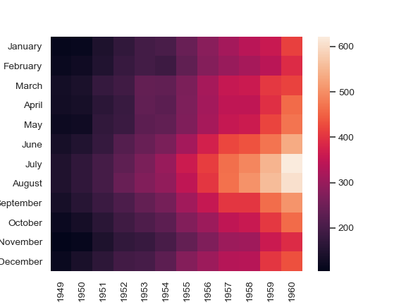
And because visualization is generally easier to understand than reading tabular data, heatmaps are typically used to visualize correlation matrices. A simple way to plot a heatmap in Python is by importing and implementing the Seaborn library.
Seaborn heatmap arguments
Seaborn heatmaps are appealing to the eyes, and they tend to send clear messages about data almost immediately. This is why this method for correlation matrix visualization is widely used by data analysts and data scientists alike.
But what else can we get from the heatmap apart from a simple plot of the correlation matrix?
In two words: A LOT.
Surprisingly, the Seaborn heatmap function has 18 arguments that can be used to customize a correlation matrix, improving how fast insights can be derived. For the purposes of this tutorial, we’re going to use 13 of those arguments.
Let’s get right to it
Getting started with Seaborn
To make things a bit simpler for the purposes of this tutorial, we’re going to use one of the pre-installed datasets in Seaborn. The first thing we need to do is import the Seaborn library and load the data.
#importing all the libraries needed
import seaborn as sns
import numpy as np
import pandas as pd
import matplotlib.pyplot as plt

tips_df = sns.load_dataset('tips')
tips_df.head()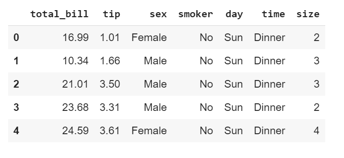
The data
Our data, which is called Tips (a pre-installed dataset on Seaborn library), has 7 columns consisting of 3 numeric features and 4 categorical features. Each entry or row captures a type of customer (be it male or female or smoker or non-smoker ) having either dinner or lunch on a particular day of the week. It also captures the amount of total bill, the tip given and the table size of a customer. (For more info about pre-installed datasets on the Seaborn library, check here)
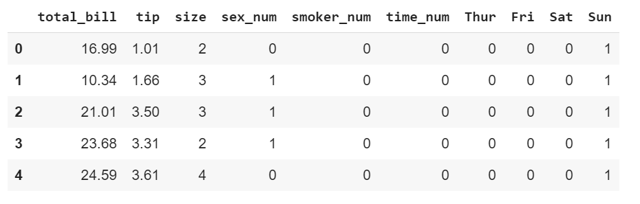
One important thing to note when plotting a correlation matrix is that it completely ignores any non-numeric column. For the purposes of this tutorial, all the category variable were changed to numeric variables.
This is how the DataFrame looks like after wrangling.
As mentioned previously, the Seaborn heatmap function can take in 18 arguments.
This is what the function looks like with all the arguments:
Just taking a look at the code and not having any idea about how it works can be very overwhelming. Let’s dissect it together.
To better understand the arguments, we’re going to group them into 4 categories:
- The Essentials
2. Adjusting the axis (the measurement bar)
3. Aesthetics
4. Changing the matrix shape
The Essentials
- The most important argument in the function is to input the data since the end goal is to plot a correlation. A .corr() method will be added to the data and passed as the first argument.
sns.heatmap(df_new.corr())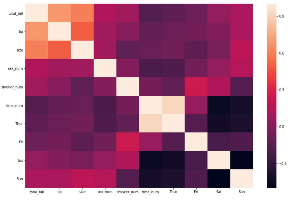
2. Interpreting the insights by just using the first argument is sufficient. For an even easier interpretation, an argument called annot=True should be passed as well, which helps display the correlation coefficient.
sns.heatmap(df_new.corr(), annot = True)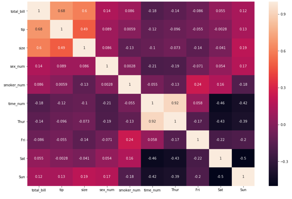
3. There are times where correlation coefficients may be running towards 5 decimal digits. A good trick to reduce the number displayed and improve readability is to pass the argument fmt =’.3g’or fmt = ‘.1g’ because by default the function displays two digits after the decimal (greater than zero) i.e fmt=’.2g’(this may not always mean it displays two decimal places). Let’s specify the default argument to fmt=’.1g’ .
sns.heatmap(df_new.corr(), annot = True, fmt='.1g')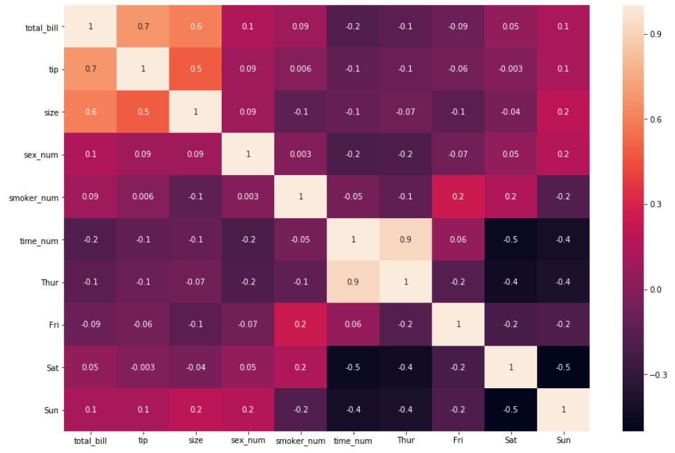
For the rest of this tutorial, we will stick to the default fmt=’.2g’
Adjusting the axis (the measurement bar)
4. The next three arguments have to do with rescaling the color bar. There are times where the correlation matrix bar doesn’t start at zero, a negative number, or end at a particular number of choice—or even have a distinct center. All this can be customized by specifying these three arguments: vmin, which is the minimum value of the bar; vmax, which is the maximum value of the bar; and center= . By default, all three aren’t specified. Let’s say we want our color bar to be between -1 to 1 and be centered at 0.
sns.heatmap(df_new.corr(), annot = True, vmin=-1, vmax=1, center= 0)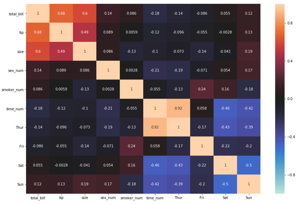
One obvious change, apart from the rescaling, is that the color changed. This has to do with changing the center from None to Zero or any other number. But this does not mean we can’t change the color back or to any other available color. Let’s see how to do this.
Aesthetic
5. Let’s change the color by specifying the argument cmap
sns.heatmap(df_new.corr(), annot = True, vmin=-1, vmax=1, center= 0, cmap= 'coolwarm')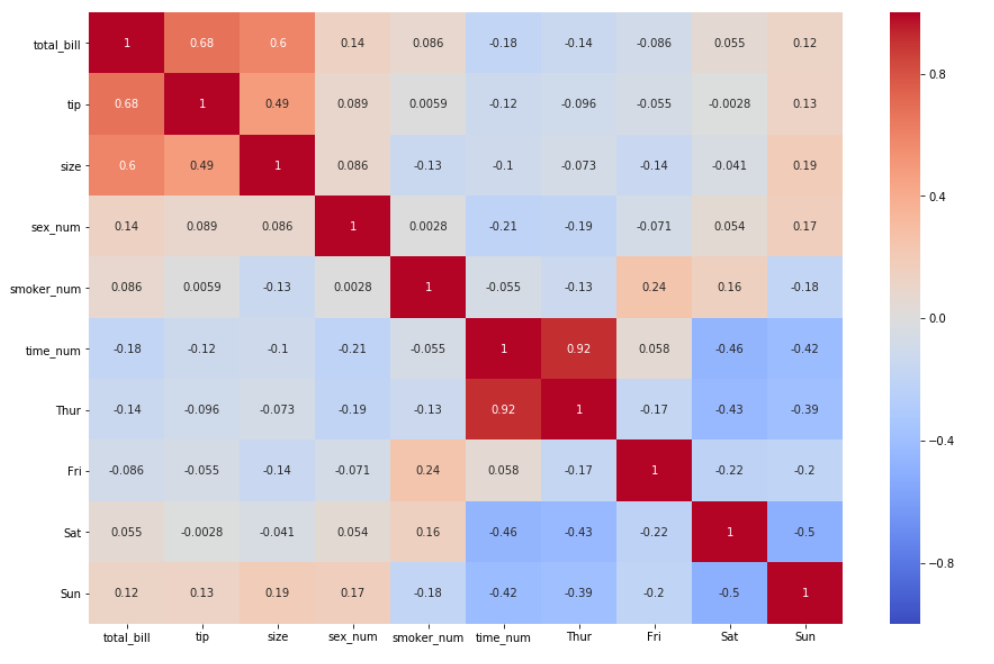
Check here for more information on the available color codes.
6. By default, the thickness and color border of each row of the matrix are set at 0 and white, respectively. There are times where the heatmap may look better with some border thickness and a change of color. This is where the arguments linewidths and linecolor apply. Let’s specify the linewidths and the linecolor to 3 and black, respectively.
sns.heatmap(df_new.corr(), annot = True, vmin=-1, vmax=1, center= 0, cmap= 'coolwarm', linewidths=3, linecolor='black')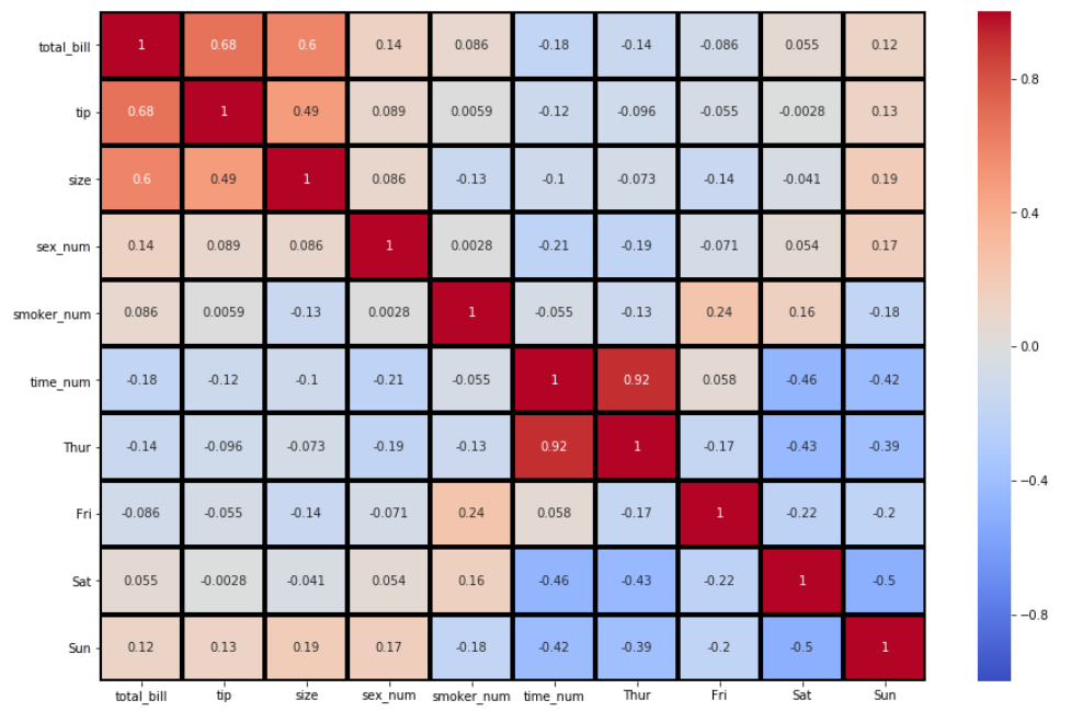
For the rest of this tutorial, we’ll switch back to the default cmap , linecolor, and linewidths . This can be done either by passing the following arguments: cmap=None , linecolor=’white’, and linewidths=0; or not passing the arguments at all (which we’re going to do).
7. So far, the heatmap used has its color bar displayed vertically. This can be customized to be horizontal instead by specifying the argument cbar_kws
sns.heatmap(df_new.corr(), annot = True, cbar_kws= {'orientation': 'horizontal'} )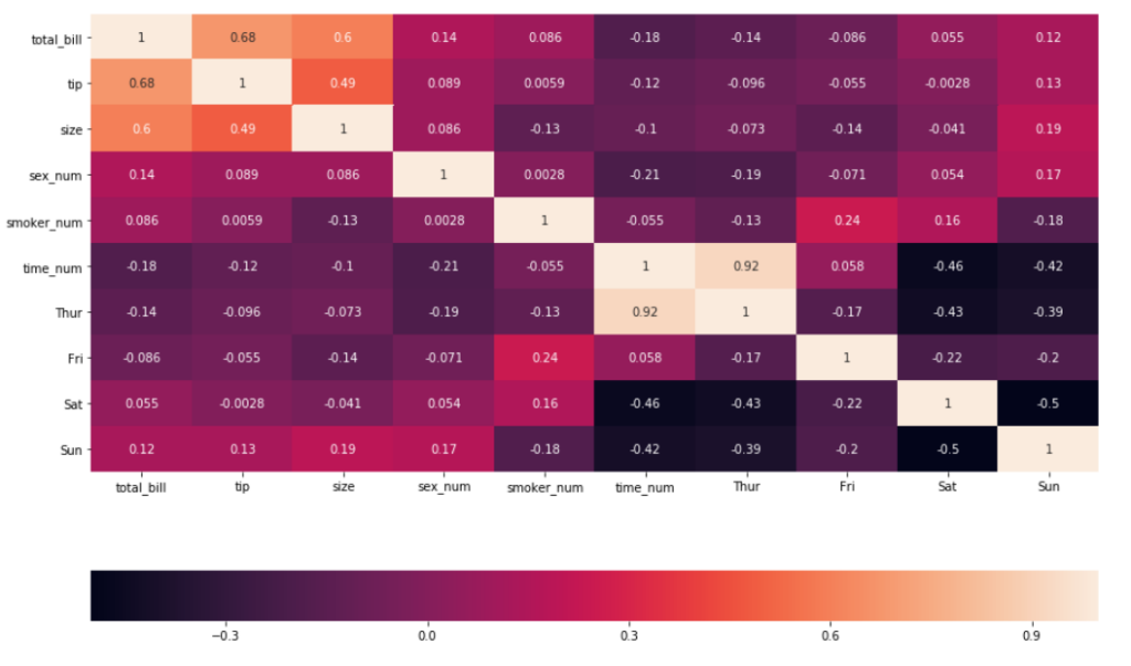
8. There also might be instances where a heatmap may be better off not having a color bar at all. This can be done by specifying cbar=False
sns.heatmap(df_new.corr(), annot = True, cbar=False)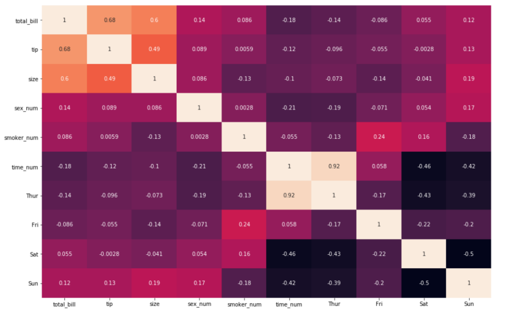
For the rest of this tutorial, we will display the color bar.
9. Take a closer look at the shape of each matrix box above. They’re all rectangular in shape. We can change them into squares by specifying the argument to square=True
sns.heatmap(df_new.corr(), annot = True,square=True)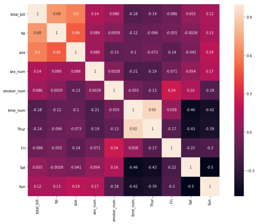
Changing the matrix shape
Changing the whole shape of the matrix from rectangular to triangular is a little tricky. For this, we’ll need to import NumPy methods .triu() & .tril() and then specify the Seaborn heatmap argument called mask=
.triu() is a method in NumPy that returns the lower triangle of any matrix given to it, while .tril() returns the upper triangle of any matrix given to it.
The idea is to pass the correlation matrix into the NumPy method and then pass this into the mask argument in order to create a mask on the heatmap matrix. Let’s see how this works below.
First using the np.trui() method:
matrix = np.triu(df_new.corr())
sns.heatmap(df_new.corr(), annot=True, mask=matrix)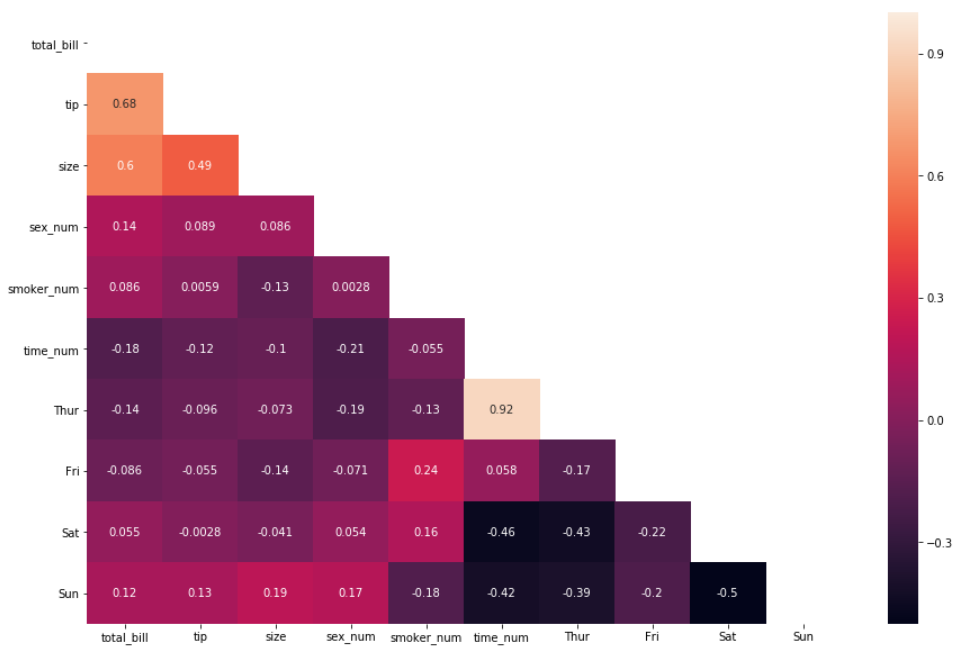
Then using the np.tril() method:
mask = np.tril(df_new.corr())
sns.heatmap(df_new.corr(), annot=True, mask=mask)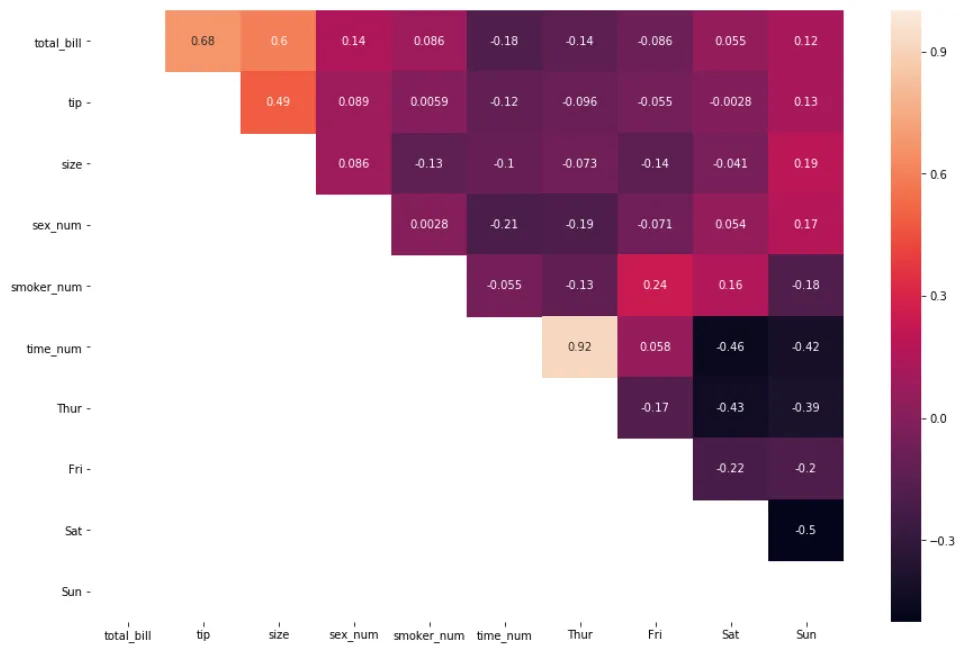
In conclusion
We discovered 13 ways to customize our Seaborn heatmap for a correlation matrix. The remaining 5 arguments are rarely used because they’re very specific to the nature of the data and the associated goals. Full source code for this tutorial can be found on GitHub:
References
Learn more about the Seaborn function using the documentation here
To learn more about improving the EDA process through visualization, check out this Dataquest tutorial (login required).

Comments 0 Responses