Research Guide: Image Quality Assessment for Deep Learning

The quality of images is relevant in building compression and image enhancement algorithms. Image Quality Assessment (IQA) is divided into two main areas; reference-based evaluation and no-reference evaluation.

Reference-based methods rely on high-quality images to evaluate the difference between two images. Structural Similarity Index is one example of a reference-based method. Unlike reference-based methods, however, no-reference methods don’t require a base image for evaluating the quality of an image. These methods just receive an image whose quality is being assessed.

In this guide, we’ll look at how deep learning has been used in image quality analysis.

Algorithm Selection for Image Quality Assessment (COSEAL 2019)

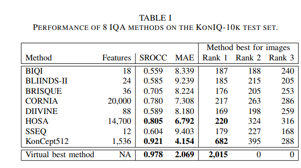
The authors of this paper compared 8 algorithms for blind IQA. They applied the AutoFolio system that trains an algorithm selector to choose the best-performing algorithm. They also trained a deep neural network to predict the best method.

A CNN is trained to classify images according to which IQA method attains the best results. InceptionResNetV2 was used for the image classification problem. It’s fine-tuned with pre-trained weights on the ImageNet dataset and was trained in 10 epochs with a batch size of 64 and a learning rate of 0.0001.

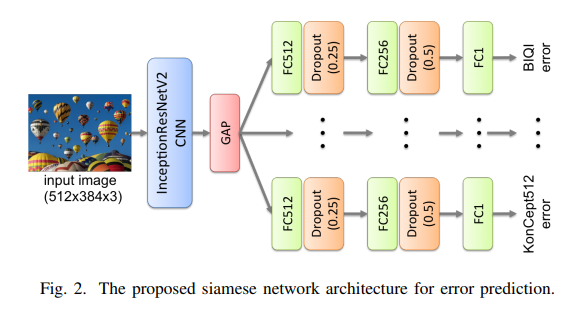
In a second approach, IQA methods M and images I, having ground truth quality values MOS(I), are considered. The error function fM(I) = M(I) − MOS(I) is formulated. These functions are trained on a Siamese neural network with a joint CNN for all methods M. The algorithm selection for a given input image first runs this network and outputs the IQA M(I) for which the network predicted the smallest fM(I).

In the architecture shown below, an image is fed into the CNN base of the InceptionResNetV2 and uses Global Average Pooling(GAP) for each feature map. The feature vector resulting from this passes through 8 separate modules. Each module predicts the error for one of the eight methods. Each module has the following layers: fully-connected (FC) with 512 units, dropout with rate 0.25, FC with 256 units, dropout with rate 0.5, and output with one neuron.

Some of the results obtained are shown below:

NIMA: Neural Image Assessment (2017)

This paper predicts the distribution of human opinion scores using a convolutional neural network. The network can be used to score images with a high correlation to human perception. It’s also useful in photo editing and enhancement. The paper aims to predict the technical and aesthetic qualities of images.

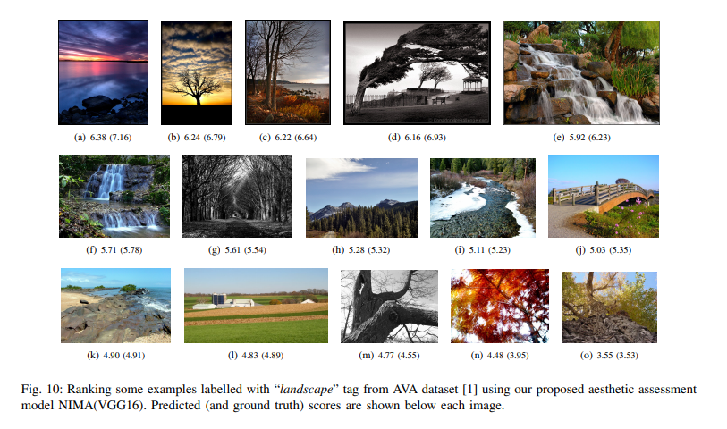
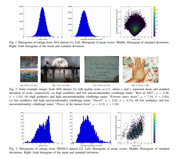
The squared EMD (earth mover’s distance) loss is used since it boosts performance in classification with ordered classes. The Aesthetic Visual Analysis (AVA) dataset is used. The AVA dataset contains about 255,000 images, rated based on aesthetic qualities by amateur photographers.

The architectures explored in this method are VGG16, Inceptionv2, and MobileNet for image quality assessment tasks. VGG16 has 13 convolutional and 3 fully-connected layers. It uses small convolutional filters of size 3 x 3. Inceptionv2 is based on the Inception module that allows for the parallel use of convolutional and pooling operations.

MobileNet is a deep CNN for mobile vision applications. For MobileNet, deep convolutional filters are replaced by separable filters. The last layer of the baseline CNN is replaced with a fully-connected layer with 10 neurons that’s followed by soft-max activations.

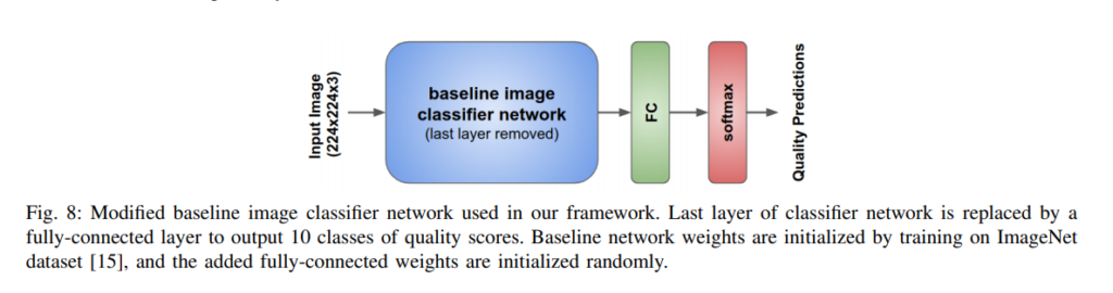
The baseline CNN weights are initialized by training on the ImageNet dataset.

Training input images are scaled to 256 × 256 and a random 224 × 224 image size is cropped. The CNNs are implemented using TensorFlow. The baseline CNN weights are initialized by training on ImageNet. The last fully-connected layer is randomly initialized.

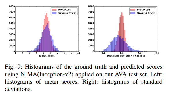
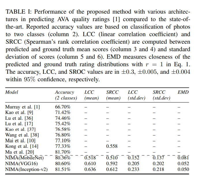
The performance of the proposed method is shown below:

Blind Image Quality Assessment Using A Deep Bilinear Convolutional Neural Network (2019)

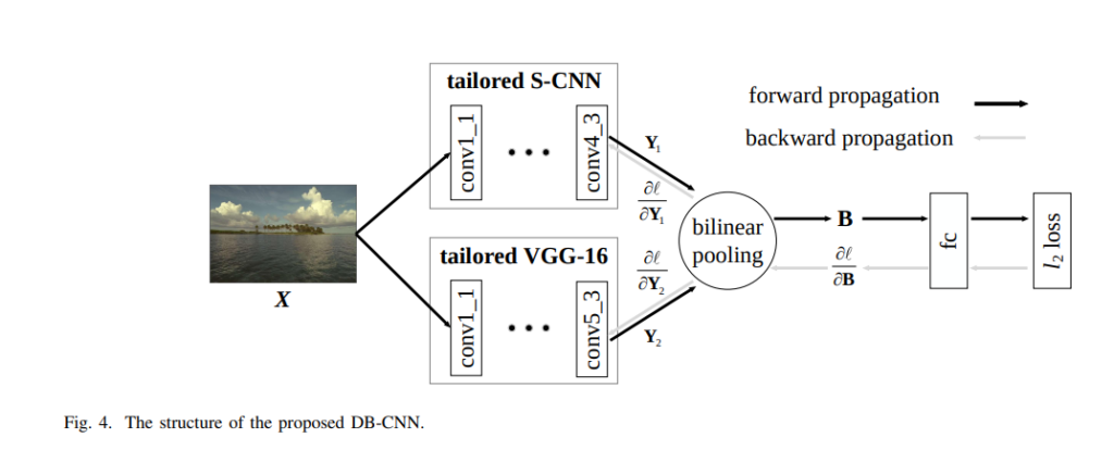
This paper proposes a deep bilinear model for blind image quality assessment(BIQA). The model consists of two convolutional neural networks. A pre-trained CNN is used to classify image distortion type and level for synthetic distortions. For authentic distortions, a pre-trained CNN is adopted for image classification. Features from the two CNNs are pooled bilinearly into a unified representation for a final quality prediction. Next, the model is fine-tuned on target subject-related databases using a variant of stochastic gradient descent.

The datasets used in this paper include Waterloo Exploration Database and the PASCAL VOC Database. The two are merged to obtain 21,869 source images. The network is designed similar to the VGG-16 network. The CNNs for synthetic distortions (S-CNN) architecture is shown below.

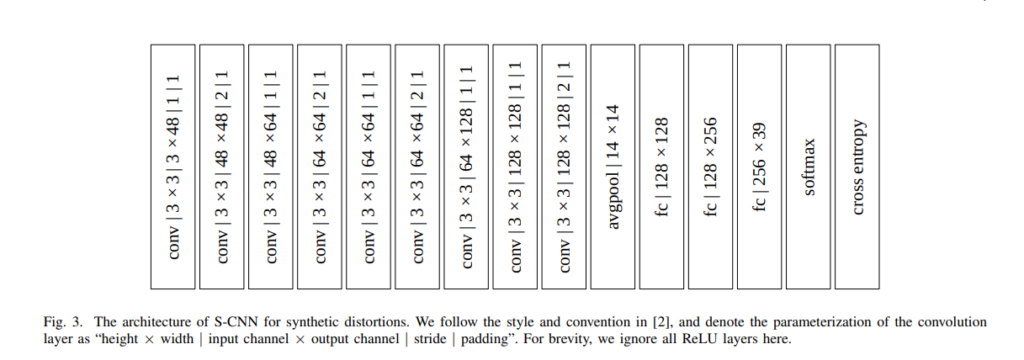
The input image is resized and cropped to 224 × 224 × 3. The convolutions have a kernel size of 3 x 3. In order to reduce the spatial resolution by half in both directions, a kernel size of two is used. The Rectified Linear Unit (ReLU) is adopted as the nonlinear activation function. Feature activations at the last convolution layer are averaged globally across spatial locations. Three fully connected layers and the softmax layer are appended at the end. For authentic distortions, a VGG-16 that had been pre-trained on ImageNet for classification is used.

For bilinear pooling, S-CNN for synthetic distortions and VGG-16 for authentic distortions are combined into a unified model. Bilinear models are more effective in modeling two-factor variations such as style and content of images, location, and appearance for fine-grained recognition, and spatial and temporal characteristics for video analysis.

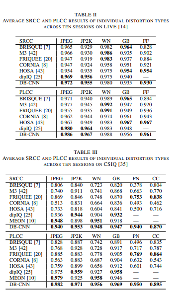
This method’s performance is shown below:

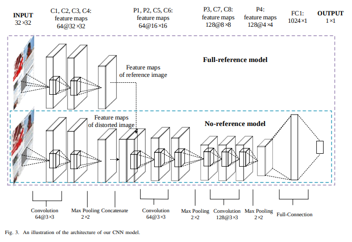
Deep Optimization Model for Screen Content Image Quality Assessment using Neural Networks (2019)

This paper proposes a quadratic optimized model based on the deep convolutional neural network (QODCNN) for screen content image quality assessment.

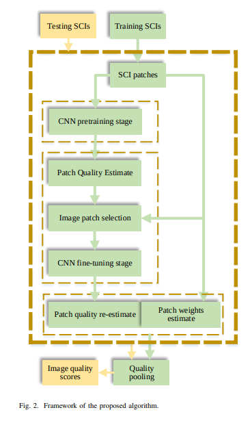
The model works in three steps. An end-to-end deep CNN is trained to predict the image visual quality in the first step. It also includes batch normalized layers and 12 regularization layers to improve the performance and speed of fitting the network. In the second step, the pre-trained model is fine-tuned to achieve better performance on raw training data. The third step involves an adaptive weighting method to fuse local quality.

Below is a representation of the QODCNN architecture. It has eight convolutional layers, four max-pooling layers, one concatenate layer, and two fully connected layers. Each convolution layer has a 3 x 3 filter with a stride of 1 pixel. Each pooling layer has a 2 x 2 pixel-sized kernel with a stride of 2 pixels. To improve network performance, zeros are padded around the border for each convolutional layer.

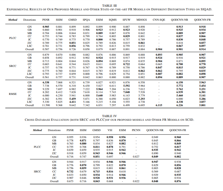
Here’s how the method performs:

Conclusion

We should now be up to speed on some of the most common — and a couple of very recent — image quality assessment methods.

The papers/abstracts mentioned and linked to above also contain links to their code implementations. We’d be happy to see the results you obtain after testing them.