Play Sheet Music with Python, OpenCV, and an Optical Music Recognition Model

Introduction

Scientists have been experimenting for some years now on ways to make computers recognize music notations. According to a paper by Jorge Calvo-Zaragoza et al, research has been done in this area of study for the past 50 years and these involved the use of different techniques most of which were based on cutting edge technology present at those times.

In recent times, these researches have evolved to the use of cutting edge computer vision technology in interpreting these music notations which have drastically reduced the research process by about half. This research area is known as Optical Music Recognition.

Optical Music Recognition is a research area that aims at giving computers the capability to recognize music notations. These can either be notations in physical/hardcopy documents in the form of handwritten notations or printed notations on paper, or digital/softcopy documents that are handwritten or digital. A more in-depth introduction to OMR can be found in the paper, linked here.

The aim of this article is to introduce you to ORM. By the end of this article, you will learn about optical music recognition, how deep learning is applied to ORM, and apply ORM in a simple music application.

OMR with Deep Learning

In this project, we’re going to be using a pre-trained deep learning model by Jorge Calvo-Zaragoza and David Rizo, built-in their research work titled End-to-End Neural Optical Music Recognition of Monophonic Scores.

Broadly speaking, they used a convolutional neural network combined with a recurrent neural network in this project. They used four convolutional layers with a 2 X 2 pooling layer, two RNN layers of 256 bidirectional long-short term memory neurons (BLSTM units), and a fully-connected layer with input neurons corresponding to the number of alphabets used in music notation, plus a neuron for the blank CTC loss function symbol (CTC loss will be discussed later).

The CNN is used to read the symbols in the input images, and the RNN to identify the symbols by dealing with the sequential nature of musical notations identified in the first stage. The output of the CNN is fed into the RNN resulting in a model that could be conveniently described as a convolutional recurrent neural network (CRNN).

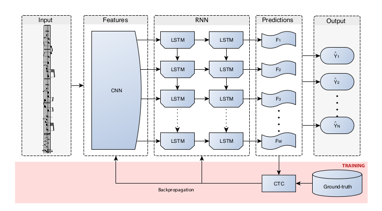
The model was trained with stochastic gradient descent (SGD), which aimed at minimizing a type of loss function called the connectionist temporal classification (CTC) loss function.

The CTC loss function is mostly used in problems where there’s no alignment between the outputs of a model and the target; for example, speech recognition problems.

The loss function works by summing up and taking the natural log of the probabilities of the different combinations of a ground-truth text, at each time step, to determine the correct output for a model. The blank symbol mentioned above is used to work with situations where there’s a repetition. The CTC loss for the word “loss ”, for example, is given by:

In their research work, the authors gathered a dataset of about 80,000 monodic single-staff sheet music scores, with each music score made up of five files: the agnostic file, semantic file, Music Encoding Initiative format file, Plaine and Easie score, and a .png file.

Intro to Common Western Modern Notation (CWMN)

In CWMN (or sheet music, as used in this article), music is represented as symbols that denote the pitch, the duration, the octave which the pitch belongs, its time signature, the key-signature, and more. The semantic vocabulary used to train our model outputs strings in English that interprets these symbols in music terms, hence the need for understanding what these terms mean. A broader introduction can be found here.

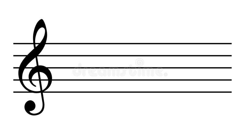
Modern CWMN is written in a staff—a set of five horizontal lines and four spaces in which the musical symbols denoting the different notes are drawn. Each line and space is named using the alphabets A – G.

Staffs are divided into bars with a vertical line across the staff. These lines are called bar lines.

Octaves are pitches whose frequencies are two times the actual frequency. In a musical staff, the octave is determined by the location of a note’s symbol on the staff.

To be able to interpret this, the OMR model’s outputs would have notes like: G4, G2, which means the note G on the fourth octave and G on the second octave. Each octave is made up of 8 notes.

Sharps # are pitches that are raised one semitone, and Flats b the ones set down by a semitone. For example, G#4, Gb2 would mean G4 raised by a semitone, and G2 lowered by a semitone.

In a piece of music, when a sharp or a flat is added to a musical note to change the note’s pitch by a semitone, it is called an accidental. The effect of accidental ends with a bar line. This means that when an accidental occurs on a music note, the pitch changes to that of a semitone wherever the notes occur in the music, except when it is changed by the opposite semitone or when it occurs in a different bar. This part is handled by the recursive neural network (RNN).

Another interesting concept that you should know is the concept of the duration of notes and rests. In CWMN, the shape of a note’s or rests symbol determines its duration. There are different types of notes, some of them are: semi-breve, crotchet, and quaver, they denote different durations. More info can be found here. A crotchet in 60bpm time has a duration of 0.5 seconds. Besides these, we have other notations that could augment the above-mentioned durations. These are fermata (or pause) and dots. The dots augments the duration of a note by half and a fermata is determined by the mood of the musician or that of the conductor of the performance but by default when a fermata occurs on a note the duration of the note is doubled. This bit is implemented in our python code in the next section.

A musical note’s pitch can be represented as a frequency; for example, the A note on the fourth octave has a frequency of 440Hz. This is achieved using a tuning system. A tuning system we will use in this project is the 12-tone-tempered system (12-TET). It is what is used to generate the contents of the dictionary we will use in the next section.

Creating Our Deep Learning Music Player

In this project, we’re going to use the simpleaudio package, OpenCV, and TensorFlow. First of all, head over to this link to download the pre-trained model that resulted from the research introduced in this article (we’re only using the semantic model in this project). And proceed to this link to clone the code that came with the OMR paper we talked about in the previous section to your device.

The idea: The OMR model outputs a string corresponding to the semantic vocabulary created by the researchers. This string output contains the description of the various notes in musical terms. This is what we’re going to use in creating our midi player. We’ll use regular expressions and a dictionary to form a sine wave array which will be interpreted by the simpleaudio package.

Let’s begin by creating two new folders in the tf-end-to-end folder and naming them midi and Models. Put the unzipped model you downloaded in the Models folder.

Assuming you’re using TensorFlow version 2.x, open the ctc_predict.py file and add the following to the top of the file.

import tensorflow.compat.v1 as tf_v1
import simpleaudio as sa
import numpy as np
from midi.player import *


tf.compat.v1.disable_eager_execution()

This is aimed at using TensorFlow version 1.x’s API (which the project was written in) in version 2.0. Now, replace tf with tf_v1 in every line of code. You can use your text editor to easily do this. Change line 51 to:

and line 54 to:

Create a file in the midi folder and name it player.py. Copy the code in the first, second, and third code snippets below into the file.

This is a break down of the code. Below is a parser that returns a music note and its duration. The function gets the string output of our model as an argument and uses Regular Expressions (regex) to extract the string associated with a note, see line 3. This is further searched with regular expressions to find the two outputs of the function: (line 7 – 10) for note’s alphabets, and (line 12 -16 ) its duration. This also uses list comprehension functionality of python to clean the result of the regex search, see line 16. You can learn more about list comprehension here.

import numpy as np
import re

from .dictionary import FREQ, DUR

def music_str_parser(semantic):
    # finds string associated with symb
    found_str = re.compile(r'((note|gracenote|rest|multirest)(-)(S)*)'
                           ).findall(semantic)
    music_str = [i[0] for i in found_str]
    # finds the note's alphabets 
    fnd_notes = [re.compile(r'(([A-G](b|#)?[1-6])|rest)'
                    ).findall(note) for note in music_str]
    # stores the note's alphabets
    notes = [m[0][0] for m in fnd_notes]
    found_durs = [re.compile(r'((_|-)([a-z]|[0-9])+(S)*)+'
                    ).findall(note) for note in music_str]
    #split by '_' every other string in list found in tuple of lists 
    durs = [i[0][0][1:].split('_') for i in found_durs]
    return notes, durs

The code below caters to special durations like fermata — which is a pause. This type of durations augments the duration of a note. This means that the augmentations are added after the actual duration has been determined. One way to achieve this is by calculating the duration of a note first and then adding these augmentations like double, quadruple, dots, double dots, or fermata after that.

At line 5, the get() function is used to return the corresponding value of a duration in seconds, it returns None for the augmentations. The augmentation is later added using the if statements after filtering None values out and summing the list, see line 8.

def dur_evaluator(durations):
    note_dur_computed = []
    for dur in durations:
        # if dur_len in DUR dict, get. Else None 
        dur_len = [DUR.get(i.replace('.','').replace('.',''), 
                              None) for i in dur]
        # filter/remove None values, and sum list
        dur_len_actual = sum(list(filter(lambda a: a !=None, 
                                      dur_len)))
        # actual duration * 4 = quadruple
        if 'quadruple' in dur:
            dur_len_actual = dur_len_actual * 4
        # actual duration * 2 = fermata
        elif 'fermata' in dur:
            dur_len_actual = dur_len_actual * 2
        # actual duration + 1/2 of duration = .
        elif '.' in ''.join(dur):
            dur_len_actual = dur_len_actual + (dur_len_actual * 1/2)
        elif '..' in ''.join(dur):
            dur_len_actual = dur_len_actual +(2 *(dur_len_actual * 1/2))
        # if no special duration string
        elif dur[0].isnumeric():
            dur_len_actual = float(dur[0]) * .5
        note_dur_computed.append(dur_len_actual)
    return note_dur_computed

The first function in the code below calculates the time-step for each second of audio using a sample rate of 44100 per second. So each second of a Note is divided into 44100 time-steps. Numpy’s linspace function is used to achieve this, see line 8. The result is appended to the list instantiated at line 4.

The nested function in the get_music_note function returns the frequency of the Notes using the alphabets of the Notes as a key to search the FREQ dictionary.

The second function computes the sine wave of each note’s frequency and its duration. This gives us the exact audio array which we will then pass to simpleaudio toLets return a playback.

def get_music_note(semantic):
    notes, durations = music_str_parser(semantic)
    sample_rate = 44100
    timestep = []
    T = dur_evaluator(durations)
    for i in T:
        # gets timestep for each sample 
        timestep.append(np.linspace(0, i, int(i * sample_rate), 
                                    False))
    def get_freq(notes):
        # get pitchs frequency from dict
        pitch_freq = [FREQ[i] for i in notes]
        return pitch_freq
    return timestep, get_freq(notes)


def get_sinewave_audio(semantic):
    audio = []
    timestep, freq = get_music_note(semantic)
    for i in range(len(freq)):
        # calculates the sinewave
        audio.append(np.sin(
            freq[i] * timestep[i] * 2 * np.pi))
    return audio

Put the following code in a separate file in the midi folder and name it vocabulary.py. It contains two dictionaries that contain the corresponding frequency of a music note from the 12 Tone Equal Tempered system (12 TET), and the duration of the music in seconds.

FREQ = { "C1": 32, "C#1": 34, "Db1": 34, "D1": 36, "D#1": 38, "Eb1": 38, "E1": 41, "F1": 43, "F#1": 46, "Gb1": 46, "G1": 49, "G#1": 52, "Ab1": 52, "A1": 55, "A#1": 58, "Bb1": 58, "B1": 61, "C2": 65, "C#2": 69, "Db2": 69, "D2": 73, "D#2": 77, "Eb2": 77, "E2": 82, "F2": 87, "F#2": 92, "Gb2": 92, "G2": 98, "G#2": 104, "Ab2": 104, "A2": 110, "A#2": 116,"Bb2": 116, "B2": 123, "C3": 130, "C#3": 138, "Db3": 138, "D3": 146, "D#3": 155, "Eb3": 155, "E3": 164, "F3": 174, "F#3": 185, "Gb3": 185, "G3": 196, "G#3":208, "Ab3":208, "A3": 220, "A#3": 233, "Bb3": 233, "B3": 246, "C4": 261,"C#4": 277, "Db4": 277, "D4": 293, "D#4": 311, "Eb4": 311, "E4": 329, "F4": 349, "F#4": 369, "Gb4": 369, "G4": 392, "G#4": 415, "Ab4": 415, "A4": 440, "A#4": 466, "Bb4": 466, "B4": 493, "C5": 523,"C#5": 554, "Db5": 554, "D5": 587, "D#5": 622, "E5": 659, "Eb5": 659, "F5": 698, "F#5": 739, "Gb5": 739, "G5": 784, "G#5": 830,"Ab5": 830, "A5": 880, "A#5": 932, "Bb5": 932, "B5": 987, "rest": 0.0067,}

DUR = {
    "double": 4.0, 
    "whole": 2.0,
    "half": 1.0,
    "quarter": .50,
    "eighth": .25,
    "sixteenth": .06,
    "thirty_second": .03,
    "sixty_fourth": .02,
    "hundred_twenty_eighth": .01,
}

To run the output of the model with our music player, add the following to the end of the ctc_predict.py file. Here, we call get_sinewave_audio, which we created in the previous step, which returns an array of sine wave frequencies to be interpreted by simpleaudio.

# form string of detected musical notes
SEMANTIC = ''
for w in str_predictions[0]:
    SEMANTIC += int2word[w] + 'n'


if __name__ == '__main__':
    # gets the audio file
    audio = get_sinewave_audio(SEMANTIC)
    # horizontally stacks the freqs    
    audio =  np.hstack(audio)
    # normalizes the freqs
    audio *= 32767 / np.max(np.abs(audio))
    #converts it to 16 bits
    audio = audio.astype(np.int16)
    #plays midi 
    play_obj = sa.play_buffer(audio, 1, 2, 44100)
    #outputs to the console
    if play_obj.is_playing():
        print("nplaying...")
        print(f'n{SEMANTIC}')  
    #stop playback when done
    play_obj.wait_done()

Then, we go to our terminal/command prompt and enter the following command:

This outputs the playback of the example music (000051652–1_2_1.png) provided in the example folder. If you want to play a different .png sheet music file, make sure you add the path to the file in the above command. Note that the model was trained on monophonic sheet music, so your music should also be monophonic for the model to perform well.

Conclusion

Congratulations on making it to the end of this article. I hope with this, I have been able to get you interested in OMR research; better still, I hope you have gotten a feel of what can be done with OMR, either in music recognition, transcribing audio or hand-written melodies to CWMN, or a novel use-case. I look forward to seeing your contributions to this area of study.