
Introduction
Naive Bayes algorithms are a set of supervised machine learning algorithms based on the Bayes probability theorem, which we’ll discuss in this article. Naive Bayes algorithms assume that there’s no correlation between features in a dataset used to train the model.
In spite of this oversimplified assumption, naive Bayes classifiers work very well in many complex real-world problems. A big advantage of naive Bayes classifiers is that they only require a relatively small number of training data samples to perform classification efficiently, compared to other algorithms like logistic regression, decision trees, and support vector machines.
Before we dive into the implementation, let’s first cover some key terms related to naive Bayes.
Key Terms
Bayes Theorem
The Bayes theorem describes the probability of a feature, based on prior knowledge of situations related to that feature. For example, if the probability of someone having diabetes is related to his or her age, then by using the Bayes theorem, the age can be used to more accurately predict the probability of diabetes.
Naive
The word naive implies that every pair of features in the dataset is independent of each other. All naive Bayes classifiers work on the assumption that the value of a particular feature is independent from the value of any other feature for a given the class.
For example, a fruit may be classified as an orange if it’s round, about 8 cm in diameter, and is orange in color. With a naive Bayes classifier, each of these three features (shape, size, and color) contributes independently to the probability that this fruit is an orange. Also, it’s assumed that there is no possible correlation between the shape, size, and color attributes.
Gaussian
Oftentimes, we deal with continuous features, and Gaussian means it’s assumed that the continuous values associated with each class are distributed according to a normal distribution. Suppose the training data contains a continuous feature A—let’s divide the feature data by the class and then find the mean and variance of x in each class—this should end up as a normal distribution.
Implementation
Let’s start our implementation using Python and a Jupyter Notebook.
Once the Jupyter Notebook is up and running, the first thing we should do is import the necessary libraries.
We need to import:
- NumPy
- Pandas
- GaussianNB
- train_test_split
- accuracy_score
- Matplotlib
To actually implement the naive Bayes classifier model, we’re going to use scikit-learn, and we’ll import our GaussianNB from sklearn.naive_bayes.
import numpy as np
import pandas as pd
from sklearn.model_selection import train_test_split
from sklearn.naive_bayes import GaussianNB
from sklearn.metrics import accuracy_score
import matplotlib.pyplot as plt
import seaborn as sns
Load the Data
Once the libraries are imported, our next step is to load the data, stored in the GitHub repository linked here. You can download the data and keep it in your local folder. After that, we can use the read_csv method of Pandas to load the data into a Pandas data frame df, as shown below:
df = pd.read_csv(‘Naive-Bayes-Classifier-Data.csv’)
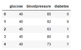
Also, in the snapshot of the data below, notice that the data frame has two columns, x and y. Here, x is the feature and y is the label. We’re going to predict y using x as an independent variable.
Data pre-processing
Before feeding the data to the naive Bayes classifier model, we need to do some pre-processing.
Here, we’ll create the x and y variables by taking them from the dataset and using the train_test_split function of scikit-learn to split the data into training and test sets.
Note that the test size of 0.25 indicates we’ve used 25% of the data for testing. random_state ensures reproducibility. For the output of train_test_split, we get x_train, x_test, y_train, and y_test values.

Train the model
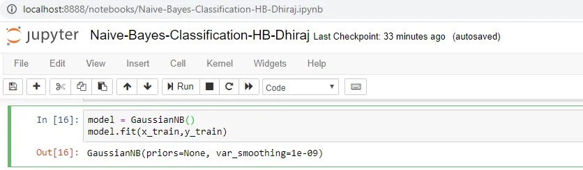
We’re going to use x_train and y_train, obtained above, to train our naive Bayes classifier model. We’re using the fit method and passing the parameters as shown below.
Note that the output of this cell is describing a few parameters like priors and var_smoothing for the model. All these parameters are configurable, and you’re free to tune them to match your requirements.
Prediction
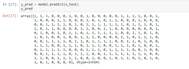
Once the model is trained, it’s ready to make predictions. We can use the predict method on the model and pass x_test as a parameter to get the output as y_pred.
Notice that the prediction output is an array of real numbers corresponding to the input array.
Model Evaluation
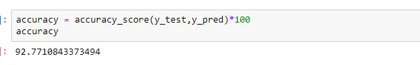
Finally, we need to check to see how well our model is performing on the test data. For this, we evaluate our model by finding the accuracy score produced by the model.
End notes
In this article, we discussed how to implement a naive Bayes classifier algorithm. We also looked at how to pre-process and split the data into features as variable x and labels as variable y.
After that, we trained our model and then used it to run predictions. You can find the data used here.

Comments 0 Responses