Machine Learning Model Evaluation & Selection

Introduction

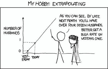
A good data scientist is not one who knows all the fancy algorithms but one who knows that he/she is overfitting. We all have been through that time when our super awesome, fully tuned model has failed to live up to the expectations on Kaggle private LB or after deployment. Knowing how to get an unbiased estimate of the predictive power of our model is important. There are different validation strategies like holdout and cross validation which are commonly used in practice for this. But which strategy is appropriate in which scenario is something that needs more discussion and thought.

In this series, I’ll share my understanding on this topic, which is derived from my experiences as a masters student in data science and many amazing blogs on this subject. This series by Sebastian Raschka was a big inspiration for this blog.

In part 1, we’ll introduce different validation strategies, their pros & cons, and how to use them correctly for model evaluation. In part 2, we’ll talk about model selection and how to bring the idea of model selection and evaluation together.

Refer to this notebook for all the codes for this post.

Outline

• Machine learning — 101
• Objectives of validation
• Holdout validation
• Cross validation

Machine learning — 101 (Back to basics)

Let’s go over some fundamental definitions in machine learning that will be commonly used.

Features & Target

Target (Y) is what we’re trying to predict. Features (X) are factors we think will help us in predicting this target.

Model

This is the manifestation of our estimate of the true (f) relationship between the features and the target.

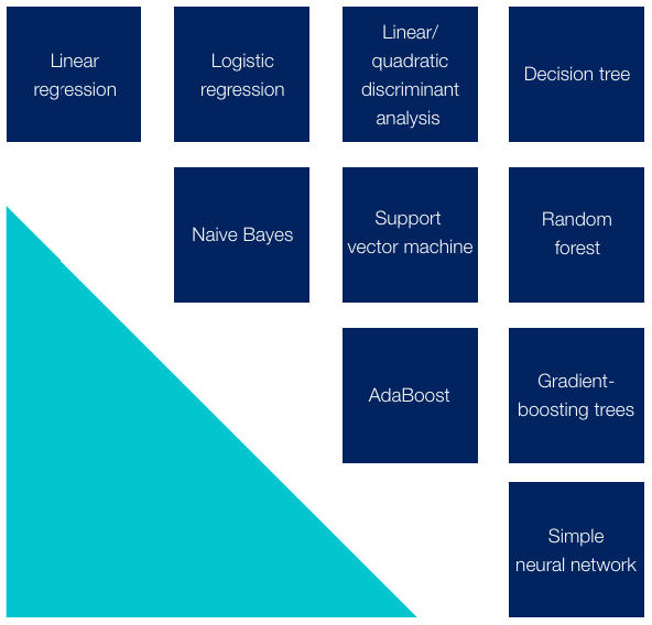
Learning algorithm

The functional space that we can explore to estimate the true relationship is infinite. The learning algorithm narrows this space. Below are some of the popular learning algorithms.

Loss/Objective function

This is a function of the difference between estimated (Ŷ) and the ground truth (Y). During training, we minimize the loss function in order to learn the functional relationship.

Parameter & Hyperparameters

Parameters of a model establish the rules of how X will translate into Ŷ. They are learnt during the model training (minimizing loss function). For ex: In regression, coefficients of features are the parameters.

Hyperparameters control how model will learn it’s parameters. They are fixed before the model training starts. For ex: k in k-nearest neighbours algorithm is a hyperparameter.

Bias & Variance

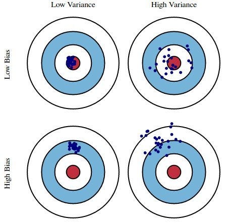
Bias and variance are general concept and are tied back to estimation of any non-deterministic parameter. Here parameter can refer to the parameters of f or true predictive power of our model. We’ll use these 2 terms in context of the latter.

High bias implies our estimate based on the observed data is not close to the true parameter. (aka underfitting).

High variance implies our estimates are sensitive to sampling. They’ll vary a lot if we compute them with a different sample of data (aka overfitting).

Now we’re ready to roll. Till now we’ve a vague idea of why we need validation. Let’s formalize this first.

Objectives of validation

We use validation strategies for 3 broad objectives:

• Algorithm selection: Selecting the class of models which is best-suited for the data at hand (tree-based models vs neural networks vs linear models)
• Hyperparameter tuning: Tuning the hyperparameters of a model to increase this predictive power
• Measure of generalizability: Computing an unbiased estimate of the predictive power of the model

We refer to the 3rd objective as model evaluation. The first 2 objectives comes under the task of model selection. We call it model selection because for a specific class of model (for ex: Random Forest) and specific values of hyperparameters (For ex: max_depth = 5), we get a single model that we train and improve. Different combinations of learning algorithms and different hyperparameters give us different models and we have to select the best among them.

In this blog, I’ll be covering model evaluation and the next blog will cover model selection.

With this in mind, let’s understand the nuances of different validation strategies. For each validation strategy, I’ll talk about the following:

• Implementation of the strategy
• Considerations while using this strategy
• Confidence intervals

Validation strategies can be broadly divided into 2 categories: Holdout validation and cross validation.

Holdout validation

Within holdout validation we have 2 choices: Single holdout and repeated holdout.

a) Single Holdout

Implementation

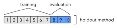
The basic idea is to split our data into a training set and a holdout test set. Train the model on the training set and then evaluate model performance on the test set. We take only a single holdout—hence the name. Let’s walk through the steps:

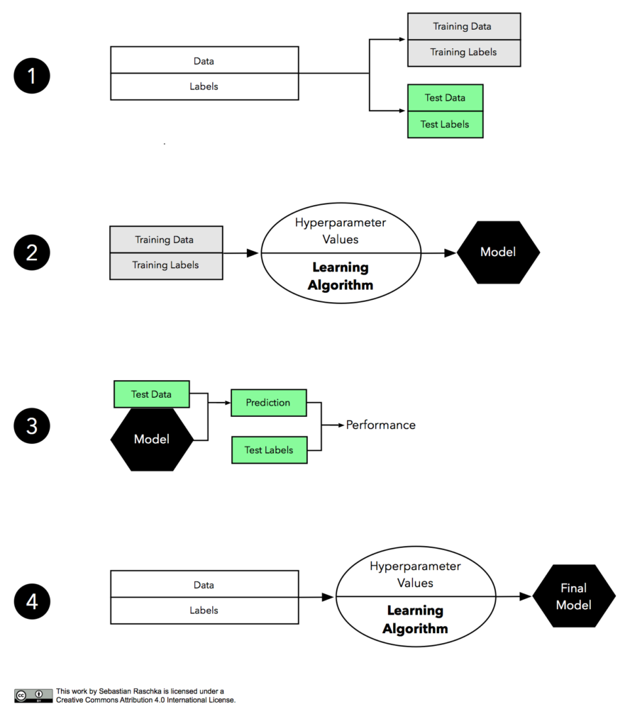
Step 1: Split the labelled data into 2 subsets (train and test).

Step 2: Choose a learning algorithm. (For ex: Random Forest). Fix values of hyperparameters. Train the model to learn the parameters.

Step 3: Predict on the test data using the trained model. Choose an appropriate metric for performance estimation (ex: accuracy for a classification task). Assess predictive performance by comparing predictions and ground truth.

Step 4: If the performance estimate computed in the previous step is satisfactory, combine the train and test subset to train the model on the full data with the same hyperparameters.

Considerations

Some things that need to be take into account while using this strategy:

Random splitting or not?

Whether to split the data randomly depends on the kind of data we have. If the observations are independent from each other, random splitting can be used. In cases where this assumption is violated, random splitting should be avoided. A typical case of this scenario is time series data, as observations are dependent on each other. For example: Today’s stock price will be dependent on yesterday’s stock price (most likely).

This also aligns with the first principle. More recent data will more likely be similar to what we can expect in production.

Stratified sampling

While splitting, we need to ensure that the distribution of features as well as target remains the same in the training and test sets.

For ex: Consider a problem where we’re trying to classify an observation as fraudulent or not. While splitting, if the majority of fraud cases went to the test set, the model won’t be able to learn the fraudulent patterns, as it doesn’t have access to many fraud cases in the training data. In such cases, stratified sampling should be done, as it maintains the proportion of different classes in the train and test set.

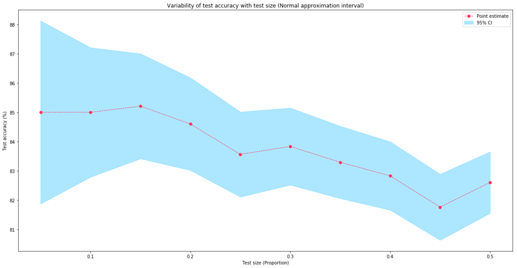
Choice of test size

Keeping aside a large amount of data for the test can result in an underestimation of predictive power (high bias**). But the estimate will be more stable (low variance**), as shown in the figure below. This consideration is more relevant for smaller datasets.

**Note: Here, bias and variance are w.r.t. the estimate of predictive power and not of the model itself.

More training data is generally better

With more training data, the model’s predictive power should improve. Therefore in step 4, we’re combining the train and test to build the final model.

No model selection

We should not do model selection and model evaluation on the same holdout. If we are trying multiple models on the same test set, we’re looking at the test set multiple times. Hence, the estimate of the true predictive power of the best model will be positively biased. More on model selection in part 2.

How confident are we in our estimates?

From the above steps, we’ll get a point estimate of the true predictive power of our model. But this single number doesn’t mean anything unless we know how confident we are in this estimate.

Defining the confidence interval around this point estimate would tell us how much this estimate can vary for a different set of model inputs. Let’s discuss a way of estimating this interval.

Normal approximation interval

Suppose we’re choosing accuracy as the proxy for predictive power of the model.

Let’s look at the calculation for the confidence interval (CI) in this case:

I used a Random Forest classifier on Fashion MNIST data (10000 images). Below is the test accuracy (single holdout) and associated 95% CI using a normal approximation interval for different test sizes.

This method not only provides a way to compute the confidence interval, but it also helps us choose an appropriate test size.

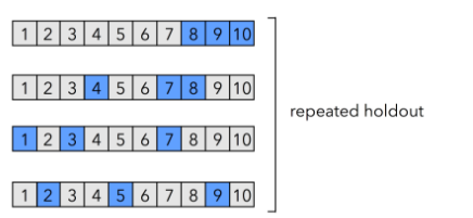
b) Repeated holdout (Monte Carlo cross validation)

Implementation

One way to obtain a more robust performance estimate that’s less variant to how we split the data is to repeat the holdout method k times with different random seeds. The estimate of predictive power of the model will be the average performance over these k repetitions. In case of accuracy as a proxy for predictive power:

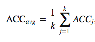
How we’re aggregating the performance over k iterations may vary with the metric we choose, but the core idea is the same.

Considerations

Apart from the points we’ve discussed for single holdout, below are some additional things to consider:

• In repeated holdout, we can test our model on a higher number of samples compared to single holdout. This reduces the variance of the final estimate.

• One more advantage of repeated holdout is that you can calculate the confidence interval empirically (discussed in the next section) instead of making distributional assumptions.
• Repeated holdout is computationally more expensive than single holdout.

How confident are we in our estimates?

Below we’ll discuss 2 ways to compute confidence interval for repeated holdout validation.

Normal approximation interval

The logic behind this is similar to what we’ve discussed for single holdout.

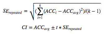
In the above formula, SE is the standard error and t is the value coming from t-distribution with degree of freedom as k-1. We’re using t-distribution because we’re calculating SE from the sample.

Empirical interval

Here we choose lower and upper bounds of the confidence interval empirically.

k-fold cross validation

Implementation

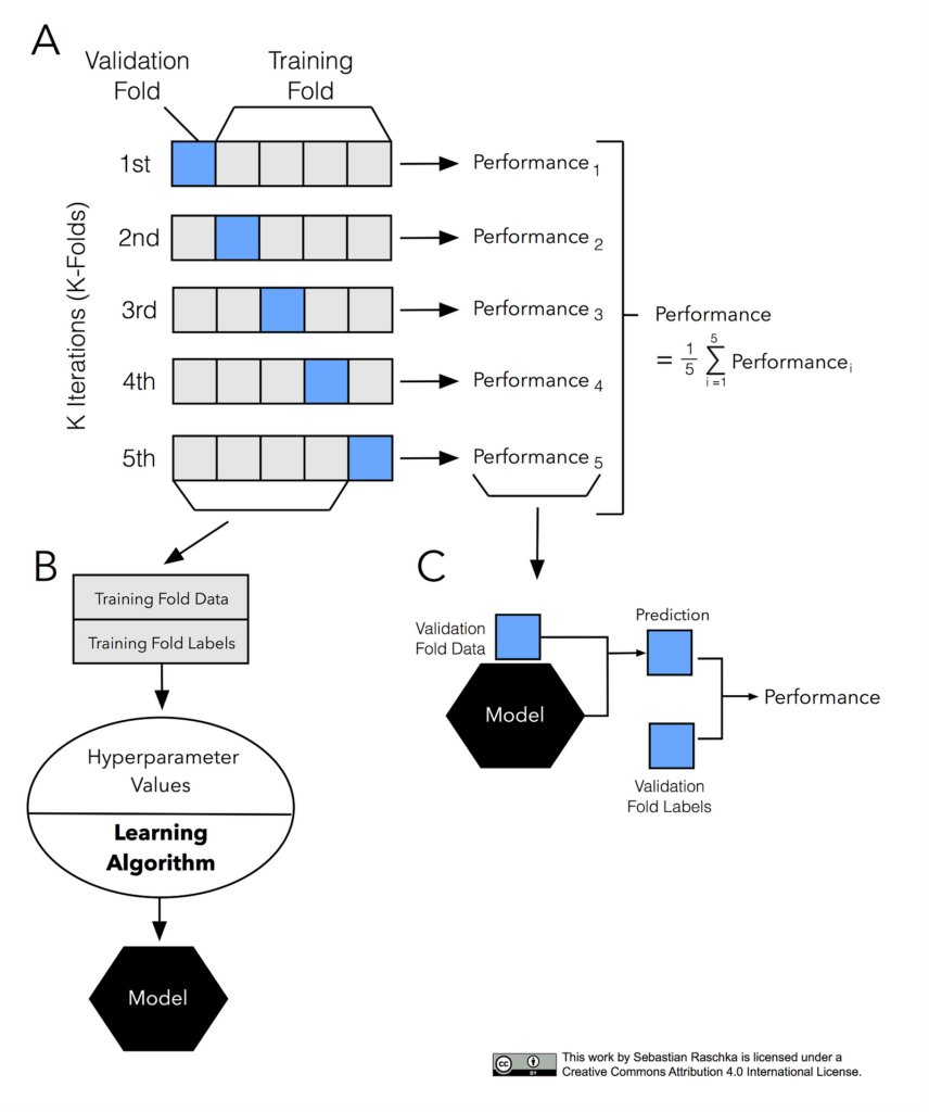
The most common approach for model evaluation is cross validation. Let’s quickly go through the steps:

• Choose a value of k and divide the data into k equal subsets
• Combine k-1 subsets and consider it as a training fold and the remaining one as a test fold
• Conduct the holdout method to get test performance (let’s choose accuracy for now)
• Repeat 2nd and 3rd steps, k times with a different subset as test fold
• Point estimate of predictive power is the average of the k different test accuracies

Considerations

• In cross-validation, every sample in our data is part of the test set exactly once. The model is tested on every sample.
• Experimental studies have suggested that cross validation estimates are less biased compared to holdout estimates.
• A special case when k = n (# of samples on data) is also called leave one out cross validation is useful when working with extremely small datasets.
• Another variation of k-fold is to repeat k-fold multiple times and take the average of performances across all the iterations. This reduces the variance further.
• Computationally less expensive than repeated holdout but more expensive than single holdout.
• For data with dependent observations like time series data, the cross validation scheme discussed above should not be used. Instead a minor modification is required, which is discussed later.

Choice of k

Small k: High bias (less data for training in each fold) but low variance (more data in test)

High k: Low bias but high variance

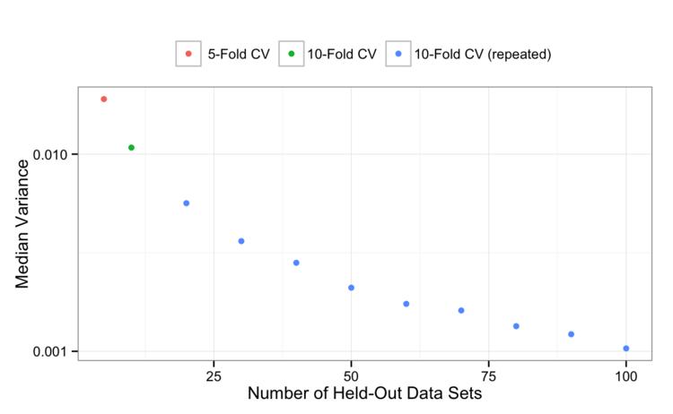
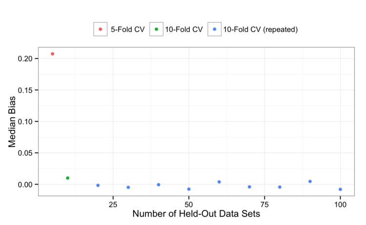
Below is the comparison of variance and bias for 5-fold CV, 10-fold CV and 10-fold CV repeated multiple times from this study.

At some point the variance will level off, but we’re still gaining precision by repeating 10-fold CV more than once.

5-fold CV is pessimistically biased, and that bias is reduced by moving to 10-fold CV. Perhaps it’s within the noise, but it would also appear that repeating 10-fold CV a few times can also marginally reduce the bias.

How confident are we in our estimates?

We can still look at the standard deviation across different folds of CV to assess the variability of CV estimate.

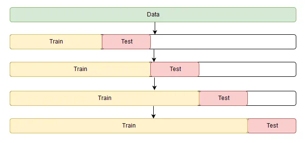
K-fold CV for time-series

Here, we first sort the data chronologically. Then for every subsequent fold, we increase the training size and test size by adding data from the next time step. Now the point estimate of the performance is the average of performances across these folds.

TL;DR

• Your testing data/environment for model evaluation should be as close to what you’re expecting post deployment. This should inspire your choice of validation strategy.
• Random splitting of data into train and test is only valid if our observations are independent.
• Stratified sampling should almost always be used for splitting the data. **In production, if we expect the distribution to be very different from what we have in our present data, stratification may not be a good choice.
• Normal approximation method/empirical method can be used to calculate confidence intervals.
• Repeated holdout is better than single holdout. It has low variance.
• Cross-validation is less biased than holdout methods (For appropriate value of k).
• k = 10 is generally a good choice for k-fold CV.
• If you’ve the computational budget, repeating 10-fold CV multiple times is a better option.
• For time-series data, temporal order should be maintained while defining the test set (Both in CV and holdout).
• If the distribution of data you expect in production is different from the data you’re building your model on (covariate shift), cross validation is not a good validation strategy. In such cases, you need to follow the holdout method and create a test set which is similar to what you’re expecting. For this, refer to links on Adversarial validation in the reference section. You can also refer to this blog which talks about how to identify covariate shift.

Next up

In part II, I’ll talk about model selection (hyperparameter tuning/algorithm selection). We’ll see modifications that we need to do in the above strategies to achieve model evaluation and selection simultaneously.

References

1. Notebook for this post
2. Blog series by Sebastian Raschka
3. How (and why) to create a good validation set by Rachel Thomas
4. Comparing Different Species of Cross-Validation
5. Improve Your Model Performance using Cross Validation

Adversarial validation

6. http://fastml.com/adversarial-validation-part-one/

7. https://github.com/zygmuntz/adversarial-validation

Discuss this post on Hacker News.