
In this article, we’ll build a simple neural network using Keras. We’ll assume you have prior knowledge of machine learning packages such as scikit-learn and other scientific packages such as Pandas and Numpy.
Training an Artificial Neural Network
Training an artificial neural network involves the following steps:
- Weights are randomly initialized to numbers that are near zero but not zero.
- Feed the observations of your dataset to the input layer.
- Forward propagation (from left to right): neurons are activated and the predicted values are obtained.
- Compare predicted results to actual values and measure the error.
- Backward propagation (from right to left): weights are adjusted.
- Repeat steps 1–5
- One epoch is achieved when the whole training set has gone through the neural network.
Business Problem
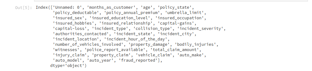
Now let’s proceed to solve a real business problem. An insurance company has approached you with a dataset of previous claims of their clients. The insurance company wants you to develop a model to help them predict which claims look fraudulent. By doing so you hope to save the company millions of dollars annually. This is a classification problem. These are the columns in our dataset.


Data Preprocessing
As in many business problems, the data provided will not be processed for us. We therefore have to prepare it in a way that our algorithm will accept it. We see from the dataset that we have some categorical columns. We need to convert these to zeros and ones so that our deep learning model will be able to understand them. Another thing to note is that we have to feed our dataset to the model as numpy arrays. Below we import the necessary packages and then load in our dataset.
We then to convert the categorical columns to dummy variables.
feats = [‘policy_state’,’insured_sex’,’insured_education_level’,’insured_occupation’,’insured_hobbies’,’insured_relationship’,’collision_type’,’incident_severity’,’authorities_contacted’,’incident_state’,’incident_city’,’incident_location’,’property_damage’,’police_report_available’,’auto_make’,’auto_model’,’fraud_reported’,’incident_type’]
df_final = pd.get_dummies(df,columns=feats,drop_first=True)
In this case we use drop_first=True to avoid the dummy variable trap. For example, if you have a, b, c, d as categories then you can drop d as a dummy variable. This is because if something does not fall into either a, b, or c then it’s definitely in d. This is referred to as multicollinearity.
We use sklearn’s train_test_split to split the data into a training set and a test set.
Next we make sure to drop the column we’re predicting to prevent it from leaking into the training set and the test set. We must avoid using the same dataset to train and test the model. We set .values at the end of the dataset in order to get the numpy arrays. This is the way our deep learning model will accept the data. This step is important because our machine learning model expects the data in form of arrays.
X = df_final.drop([‘fraud_reported_Y’,’policy_csl’,’policy_bind_date’,’incident_date’],axis=1).values
y = df_final[‘fraud_reported_Y’].values
We then split the data into a training and test set. We use 0.7 of the data for training and 0.3 for testing.
Next we have to scale our dataset using Sklearn’s StandardScaler. Due to the massive amounts of computations taking place in deep learning, feature scaling is compulsory. Feature scaling standardizes the range of our independent variables.
Building the Artificial Neural Network(ANN)
The first thing we need to do is import Keras. By default, Keras will use TensorFlow as its backend.
Next we need to import a few modules from Keras. The Sequential module is required to initialize the ANN, and the Dense module is required to build the layers of our ANN.
Next we need to initialize our ANN by creating an instance of Sequential. The Sequential function initializes a linear stack of layers. This allows us to add more layers later using the Dense module.
Adding input layer (First Hidden Layer)
We use the add method to add different layers to our ANN. The first parameter is the number of nodes you want to add to this layer. There is no rule of thumb as to how many nodes you should add. However, a common strategy is to choose the number of nodes as the average of nodes in the input layer and the number of nodes in the output layer.
Say for example you had five independent variables and one output. Then you would take the sum of that and divide by two, which is three. You can also decide to experiment with a technique called parameter tuning. The second parameter, kernel_initializer, is the function that will be used to initialize the weights.
In this case, it will use a uniform distribution to make sure that the weights are small numbers close to zero. The next parameter is the activation function. We use the Rectifier function, shortened as ReLU. We mostly use this function for the hidden layer in ANN. The final parameter is input_dim, which is the number of nodes in the input layer. It represents the number of independent variables.
Adding Second Hidden Layer
Adding the second hidden layer is similar to adding the first hidden layer.
We don’t need to specify the input_dim parameter because we have already specified it in the first hidden layer. In the first hidden layer, we specified this in order to let the layer know how many input nodes to expect. In the second hidden layer the ANN already knows how many input nodes to expect so we don’t need to repeat ourselves.
Adding the output layer
We change the first parameter because in our output node we expect one node. This is because we are only interested in knowing whether a claim was fraudulent or not. We change the activation function because we want to get the probabilities that a claim is fraudulent. We do this by using the Sigmoid activation function.
In case you’re dealing with a classification problem that has more than two classes (i.e. classifying cats, dogs, and monkeys) we’d need to change two things. We’d change the first parameter to 3 and change the activation function to softmax. Softmax is a sigmoid function applied to an independent variable with more than two categories.
Compiling the ANN
Compiling is basically applying a stochastic gradient descent to the whole neural network. The first parameter is the algorithm you want to use to get the optimal set of weights in the neural network. The algorithm used here is a stochastic gradient algorithm.
There are many variants of this. A very efficient one to use is Adam. The second parameter is the loss function within the stochastic gradient algorithm. Since our categories are binary, we use the binary_crossentropy loss function. Otherwise we would have used categorical_crossentopy. The final argument is the criterion we’ll use to evaluate our model. In this case we use the accuracy.
Fitting our ANN to the training set
X_train represents the independent variables we’re using to train our ANN, and y_train represents the column we’re predicting. Epochs represents the number of times we’re going to pass our full dataset through the ANN. Batch_size is the number of observations after which the weights will be updated.
Predicting using the training set
This will show us the probability of a claim being fraudulent. We then set a threshold of 50% for classifying a claim as fraudulent. This means that any claim with a probability of 0.5 or more will be classified as fraudulent.
This way the insurance firm can be able to first track claims that are not suspicious and then take more time evaluating claims flagged as fraudulent.
Checking the confusion matrix
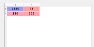
The confusion matrix can be interpreted as follows. Out of 2000 observations, 1550 + 175 observations were correctly predicted while 230 + 45 were incorrectly predicted. You can calculate the accuracy by dividing the number of correct predictions by the total number of predictions. In this case (1550+175) / 2000, which gives you 86%.
Making a single Prediction
Let’s say the insurance company gives you a single claim. They’d like to know if the claim is fraudulent. What would you do to find out?
where a,b,c,d represents the features you have.
Since our classifier expects numpy arrays, we have to transform the single observation into a numpy array and use the standard scaler to scale it.
Evaluating our ANN
After training the model one or two times, you’ll notice that you keep getting different accuracies. So you’re not quite sure which one is the right one. This introduces the bias variance trade off. In essence, we’re trying to train a model that will be accurate and not have too much variance of accuracy when trained several times.
To solve this problem we use the K-fold cross validation with K equal to 10. This will split the training set into 10 folds. We’ll then train our model on 9 folds and test it on the remaining fold. Since we have 10 folds, we’re going to do this iteratively through 10 combinations. Each iteration will gives us its accuracy. We’ll then find the mean of all accuracies and use that as our model accuracy. We also calculate the variance to ensure that it’s minimal.
Keras has a scikit learn wrapper (KerasClassifier) that enables us to include K-fold cross validation in our Keras code.
Next we import the k-fold cross validation function from scikit_learn
The KerasClassifier expects one of its arguments to be a function, so we need to build that function.The purpose of this function is to build the architecture of our ANN.
def make_classifier():
    classifier = Sequential()
    classiifier.add(Dense(3, kernel_initializer = ‘uniform’, activation = ‘relu’, input_dim=5))
    classiifier.add(Dense(3, kernel_initializer = ‘uniform’, activation = ‘relu’))
    classifier.add(Dense(1, kernel_initializer = ‘uniform’, activation = ‘sigmoid’))
    classifier.compile(optimizer= ‘adam’,loss = ‘binary_crossentropy’,metrics = [‘accuracy’])
    return classifier
This function will build the classifier and return it for use in the next step. The only thing we have done here is wrap our previous ANN architecture in a function and return the classifier.
We then create a new classifier using K-fold cross validation and pass the parameter build_fn as the function we just created above. Next we pass the batch size and the number of epochs, just like we did in the previous classifier.
To apply the k-fold cross validation function we can use scikit-learn’s cross_val_score function. The estimator is the classifier we just built with make_classifier and n_jobs=-1 will make use of all available CPUs. cv is the number of folds and 10 is a typical choice. The cross_val_score will return the ten accuracies of the ten test folds used in the computation.
To obtain the relative accuracies we get the mean of the accuracies.
The variance can be obtained as follows:
The goal is to have a small variance between the accuracies.
Fighting Overfitting
Overfitting in machine learning is what happens when a model learns the details and noise in the training set such that it performs poorly on the test set. This can be observed when we have huge differences between the accuracies of the test set and training set, or when you observe a high variance when applying k-fold cross validation.
In artificial neural networks, we counteract this using a technique called dropout regularization. Dropout regularization works by randomly disabling some neurons at each iteration of the training to prevent them from being too dependent on each other.
from keras.layers import Dropout

classifier = Sequential()
classiifier.add(Dense(3, kernel_initializer = ‘uniform’, activation = ‘relu’, input_dim=5))

# Notice the dropouts
classifier.add(Dropout(rate = 0.1))
classiifier.add(Dense(6, kernel_initializer = ‘uniform’, activation = ‘relu’))
classifier.add(Dropout(rate = 0.1))

classifier.add(Dense(1, kernel_initializer = ‘uniform’, activation = ‘sigmoid’))
classifier.compile(optimizer= ‘adam’,loss = ‘binary_crossentropy’,metrics = [‘accuracy’])
In this case we apply the dropout after the first hidden layer and after the second hidden layer. Using a rate of 0.1 means that 1% of the neurons will be disabled at each iteration. It is advisable to start with a rate of 0.1. However you should never go beyond 0.4 because you will now start to get underfitting.
Parameter Tuning
Once you obtain your accuracy you can tune the parameters to get a higher accuracy. Grid Search enables us to test different parameters in order to obtain the best parameters.
The first step here is to import the GridSearchCV module from sklearn.
We also need to modify our make_classifier function as follows. We create a new variable called optimizer that will allow us to add more than one optimizer in our params variable.
def make_classifier(optimizer):
    classifier = Sequential()
    classiifier.add(Dense(6, kernel_initializer = ‘uniform’, activation = ‘relu’, input_dim=11))
    classiifier.add(Dense(6, kernel_initializer = ‘uniform’, activation = ‘relu’))
    classifier.add(Dense(1, kernel_initializer = ‘uniform’, activation = ‘sigmoid’))
    classifier.compile(optimizer= optimizer,loss = ‘binary_crossentropy’,metrics = [‘accuracy’])
    return classifier
We’ll still use the KerasClassifier, but we won’t pass the batch size and number of epochs since these are the parameters we want to tune.
The next step is to create a dictionary with the parameters we’d like to tune — in this case the batch size, the number of epochs, and the optimizer function. We still use Adam as an optimizer and add a new one called rmsprop. The Keras documentation recommends rmsprop when dealing with Recurrent Neural Networks. However we can try it for this ANN to see if it gives us a better result.
We then use Grid Search to test these parameters. The grid search function expects our estimator, the parameters we just defined, the scoring metric and the number of k-folds.
Like in previous objects we need to fit our training set.
We can get the best selection of parameters using best_params from the grid search object. Likewise we use the best_score_ to get the best score.
It’s important to note that this process will take a while as it searches for the best parameters.
Conclusion
Artificial Neural Networks are just one type of deep neural network. There are other networks such Recurrent Neural Networks (RNN), Convolutional Neural Networks(CNN), and Boltzmann machines.
RNNs can predict if the price of a stock will go up or down in the future. CNNs are used in computer vision — recognizing cats and dogs in a set of images or recognizing the presence of cancer cells in a brain image. Boltzmann machines are used in programming recommender systems. Maybe we can cover one of these neural networks in the future.
Discuss this post on Hacker News
Comments 0 Responses