
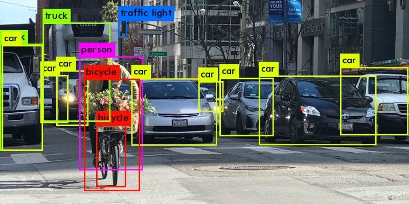
Object detection is a technology related to computer vision and image processing that deals with detecting and locating instances of semantic objects of a certain class (such as humans, buildings, or cars) in digital images and videos.
In this post, we’ll briefly discuss feature descriptors, and specifically Histogram of Oriented Gradients (HOG). We’ll also provide an overview of deep learning approaches to about object detection, including Region-based Convolutional Neural Networks (RCNN) and YOLO(you only look once).
Let’s get started!
Histogram of Oriented Gradients
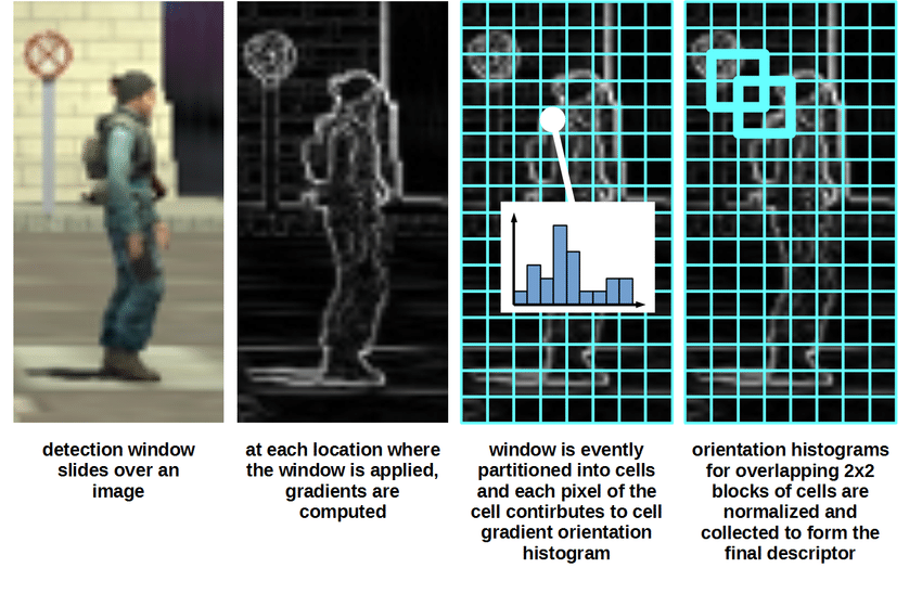
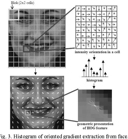
Histogram of oriented gradients (HOG) is a feature descriptor. A feature descriptor is a representation of an image—or parts of an image known as patches—that extracts useful information for the model to interpret, such as crucial information in the image like a human or textual data and ignores the background. As such, HOGs and can be used effectively in object detection.
Typically, a feature descriptor converts an image of size width x height x 3 (number of channels) to a feature vector / array of length n. In the case of the HOG feature descriptor, the input image is of size 64 x 128 x 3, and the output feature vector is of length 3780, which were the dimensions of the original paper, in which HOG was introduced.
For more details, have a look at this research paper.
Implementation of the HOG descriptor:
Step 1- Preprocessing
As mentioned earlier, the HOG feature descriptor is calculated on a 64×128 patch of an image, and you need to maintain an aspect ratio of 1:2.
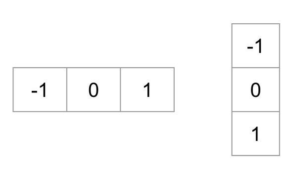
Step 2- Gradient calculation
We need to calculate gradients by passing the image through these kernels, for gradients in both horizontal and vertical directions.
The magnitude of the gradient fires wherever there’s a sharp change in intensity of the pixels. None of them fire when the region is smooth.
The gradient image removes a lot of unnecessary and extraneous information like the background, but highlights outlines of the major objects.
At every pixel, the gradient has a magnitude and a direction.
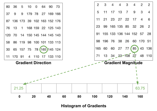
Step 3- Calculation of Histogram of Gradients
An 8×8 image patch contains 8x8x3 = 192 pixel values. The gradient of this patch contains 2 values (magnitude and direction) per pixel, which adds up to 8x8x2 = 128.
The histogram is essentially a vector of 9 bins (numbers) corresponding to angles 0, 20, 40, 60 … 160.
The contributions of all the pixels in the 8×8 cells are added up in a sliding window fashion to create the 9-bin histogram.
Step 4- Normalize and Visualize the Output
Gradients of an image are sensitive to variations in lighting effects. Ideally, we want our descriptor to be independent of lighting variations. Thus, we should “normalize” the histogram so the gradients aren’t affected by lighting variations.
To calculate the final feature vector for the entire image patch, the 36×1 vectors are concatenated into one giant vector.
A simple implementation of HOG can be found in the Python package called “skimage”. Just two lines. It’s that simple! Have a look:
So to sum it up:
- Divide the image into small patches called cells or grids, and for each cell compute a histogram of gradients for the pixels within the cell.
- Discretize each cell into angular bins according to the gradient orientation.
- Each cell’s pixel contributes weighted gradient to its corresponding angular bin.
- A normalized group of histograms represents the block histogram. The set of these block histograms represents the descriptor.
Now that we’ve looked into feature descriptors, it’s time to see how object detection algorithms are used with neural networks.
Object Detection Algorithms for Neural Networks
Object detection has always been an interesting problem in the field of deep learning. Its primarily performed by employing convolutional neural networks (CNNs), and specifically region-based CNNs (R-CNNs).
R-CNNs(Region based CNNs)
Instead of working on a massive number of regions,or going through each and every pixel and localised part of the image to search for the presence of an object, the R-CNN algorithm proposes a bunch of boxes within an input image and checks to see if any of these boxes contain any object. R-CNN then uses selective search to extract these boxes from an image.
Issues with R-CNNs
Training an R-CNN model is expensive and slow because:
- We must extract 2,000 regions for each image based on selective search
- We also have to extract features using a CNN for every image region. Suppose we have N images—the number of CNN features will be N*2,000
These processes combine to make R-CNN very slow. It takes around 40–50 seconds to make predictions for each new image, which essentially makes the model cumbersome and practically impossible to build when faced with a gigantic dataset.
A better alternative: YOLO
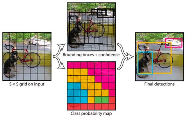
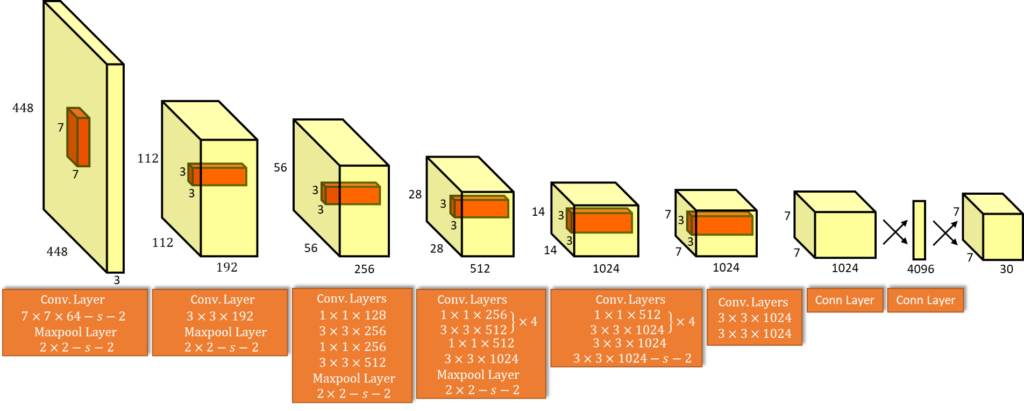
YOLO’s architecture is based on CNNs using anchor boxes and is proven to be the go-to object detection technique for a wide range of problems like detection of vehicles on the road for traffic monitoring, detection of humans in an image etc. YOLO employs an F-CNN (fully convolutional neural network). It passes an input image (nxn) once through the F-CNN and outputs a prediction (mxm).
Thus, the architecture is splitting the input image in an mxm grid, and for each grid, generates 2 bounding boxes and class probabilities for those bounding boxes.
Bounding boxes contain potential objects and the class probabilities that correspond to the object’s class.
From the original paper-
High-scoring regions of the image are considered detections.
For reference, here is the link to the original paper.
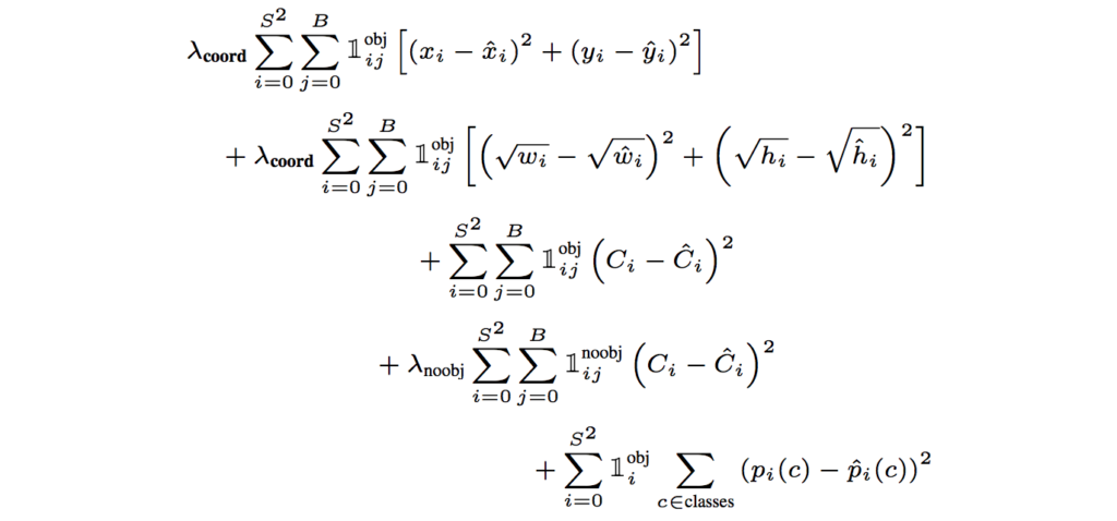
YOLO’s Loss function
YOLO predicts multiple bounding boxes per grid cell. To compute the loss for the true positive, we only want one of them to be responsible for the object. For this purpose, we select the box with the highest IoU (Intersection Over Union) with the ground truth.
YOLO uses sum-squared error between the predictions and the ground truth to calculate loss. The loss function is composed of:
- the classification loss.
- the localization loss (errors between the predicted bounding box and the ground truth).
- the confidence loss (the object-ness of the box).
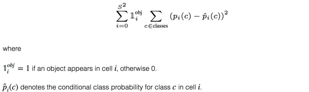
Classification loss
For every object detected, the classification loss at each cell is the squared error of the class conditional probabilities for each class:
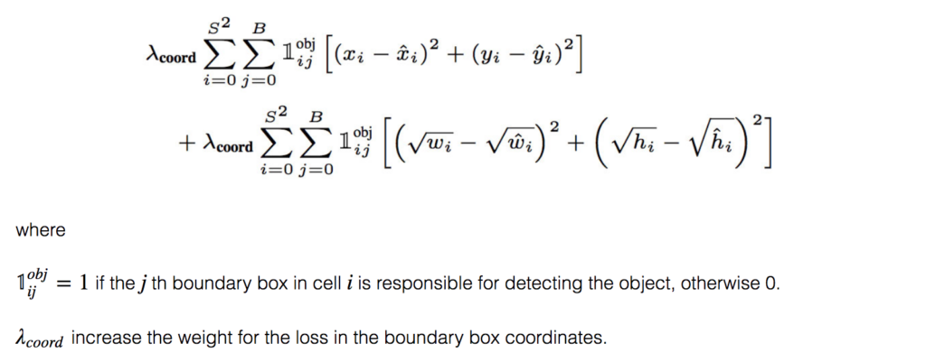
Localization loss
The localization loss measures the difference between the predicted bounding box locations and sizes.
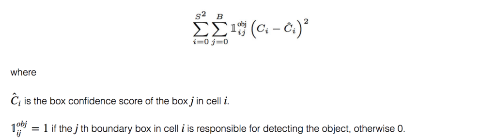
Confidence loss
If an object is detected in the box, the confidence loss (measuring the object-ness of the box) is:
If an object is not detected in the box, the confidence loss is:
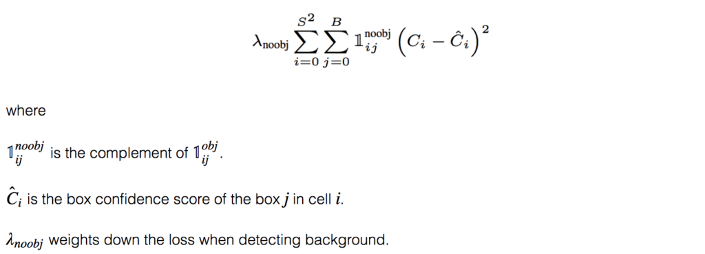
Due to a problem of imbalance—i.e. since most of the boxes do not contain any objects or most of the bounding boxes will possess just a part of the object or just background noise—we train the model to detect backgrounds more frequently than objects. To remedy this, we weight this loss down by a factor λnoobj (default: 0.5).
Final Loss
The final loss adds localization, confidence, and classification losses together.
Advantages of YOLO
- YOLO is fast and efficient for real-time processing.
- YOLO detects one object per grid cell. Thus, it introduces spatial diversity in making predictions, and all the predictions are made with one pass of the network.
- Predictions or detections are made from a single network. Thus, YOLO can be trained end-to-end to improve accuracy.
Limitations of YOLO
- YOLO imposes strong spatial constraints on bounding box predictions. Each grid can only predict two boxes and one class. Thus, detecting smaller objects that appear in groups becomes difficult.
- Newer or unusual aspect ratios for bounding boxes is hard to find for the network.
- A small error in a large box is generally fine, but a small error in a small box has a much greater effect on IOU (Intersection Over Union). Our main source of error is thus incorrect localizations.
Interesting sources to start working with these algorithms
For HOG-
For YOLO-
Conclusion
In this post, we outlined the two most commonly applied algorithms in object detection—HOG and YOLO. HOG is a feature descriptor that has been proven to work well with SVM and similar machine learning models, whereas YOLO is employed by deep learning-based neural networks. There are instances where these algorithms work well—on the other hand, rigorous research in object detection is underway to more efficiently efficiently employ it in real time.
All this effort for a machine to see through our eyes!

Comments 0 Responses