Implementing Multiple Linear Regression Using sklearn

Introduction

As an exercise, or even to solve a relatively simple problem, many of you may have implemented linear regression with one feature and one target. However, in the real world, most machine learning problems require that you work with more than one feature.

For example, to calculate an individual’s home loan eligibility, we not only need his age but also his credit rating and other features.

In other words, if you want to determine whether or not this person should be eligible for a home loan, you’ll have to collect multiple features, such as age, income, credit rating, number of dependents, etc.

So in this post, we’re going to learn how to implement linear regression with multiple features (also known as multiple linear regression). We’ll be using a popular Python library called sklearn to do so.

You may like to watch a video on Multiple Linear Regression as below.

Prerequisite Libraries

We need to have access to the following libraries and software:

1. Python 3+ → Python is an interpreted, high-level, general-purpose programming language.
2. Pandas → Pandas is a Python-based library written for data manipulation and analysis.
3. NumPy → NumPy is a Python-based library that supports large, multi-dimensional arrays and matrices. Also, NumPy has a large collection of high-level mathematical functions that operate on these arrays.
4. sklearn → sklearn is a free software machine learning library for Python.

As you can see below, we’ve imported the required libraries into our Jupyter Notebook.

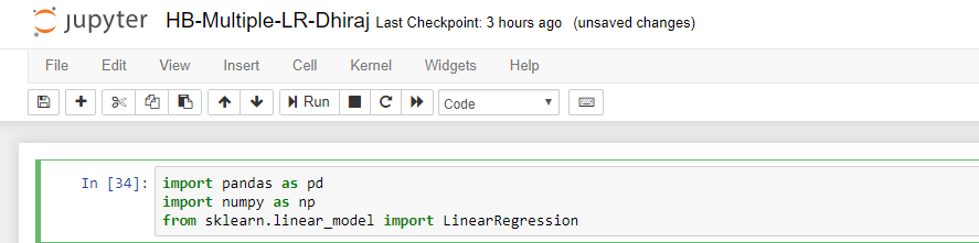
Note that we’re also importing LinearRegression from sklearn.linear_model. LinearRegression fits a linear model with coefficients to minimize the root mean square error between the observed targets in the dataset and the targets predicted by the linear approximation.

Loading the data

Now it’s time to load our data into a Pandas dataframe. For this, we’ll use Pandas’ read_csv method. We’ve stored the data in .csv format in a file named multiple-lr-data.csv. Let’s use the head() method in Pandas to see the top 5 rows of the dataframe.

Note that the data has four columns, out of which three columns are features and one is the target variable.

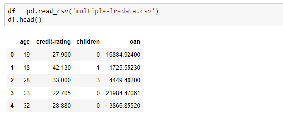
In the above data, we have age, credit-rating, and number of children as features and loan amount as the target variable.

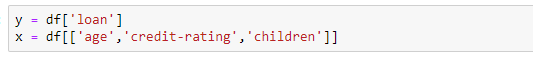
Separate the features and target

Before implementing multiple linear regression, we need to split the data so that all feature columns can come together and be stored in a variable (say x), and the target column can go into another variable (say y).

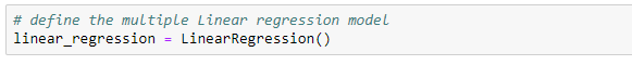
Define the Model

After we’ve established the features and target variable, our next step is to define the linear regression model. For this, we’ll create a variable named linear_regression and assign it an instance of the LinearRegression class imported from sklearn.

Linear regression is one of the fundamental algorithms in machine learning, and it’s based on simple mathematics. Linear regression works on the principle of formula of a straight line, mathematically denoted as y = mx + c, where m is the slope of the line and c is the intercept. x is the the set of features and y is the target variable.

Fit the Model

After defining the model, our next step is to train it. We re going to use the linear_regression.fit method provided by sklearn to train the model. Note that we’re passing variables x and y, created in an earlier step, to the fit method.

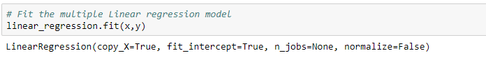
Let’s dig a bit deeper into the four parameters of linear regression, as shown above:

• copy_x is a boolean parameter. It’s optional, and the default value of this parameter is True. If True, x will be copied; otherwise, x may be overwritten.
• fit_intercept is a boolean parameter. It’s optional and the default value of this parameter is True. If set to False, no intercept will be used in the calculations (i.e. data is expected to be centered).
• n_jobs is an integer value parameter. It can also take a value of None. It’s optional and the default value of this parameter is None. n_jobs is the count of the number of jobs to be used for computation.
• normalize is a boolean parameter. It is optional and default value of this parameter is False. This parameter is ignored when fit_intercept is set to False. If True, the regressors x will be normalized before regression.

Predict

In this step, we’ll be using the model to predict the target values for given features. The input to the predict function will be the feature variable x and the output will be a variable y_pred that will contain all the predictions generated by the model.

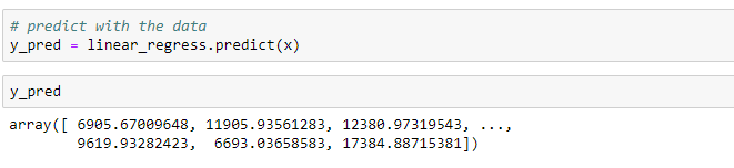
Note that the y_pred is an array with a prediction value for each set of features.

End Notes

In this article, we saw how to implement linear regression in cases where we have more than one feature. We also looked at how to collect all the features in a single variable x and target in another variable y.

After that, we trained our model and then used it to run predictions as well. You can find the code and data here.

Thanks for reading. Happy Coding!

You may like to check, how to implement Linear Regression from Scratch