Hands-on with Feature Engineering Techniques: Variables Types

This post is a part of a series about feature engineering techniques for machine learning with python.

You can check out the rest of the articles below — links will be added as posts go live:

Welcome back! Part two in our series intends to give you an overview of the type variable, which you can find in a given dataset. It’s essential to know the different variables’ types to better to engineer them.

What is a Variable?

A variable is any characteristic, number, or quantity that can be measured or counted. We call them variables because the values they take may vary, and usually do.

The following are examples of variables:

Age (23, 52, 60, …).
Gender (male, female)
Country of birth (Algeria, USA, Japan, …)
Eye color (green, brown, blue, and purple maybe)
Vehicle Brand (Buggati, Ferrari)

We classify variables in a dataset into one of these major types:

Numerical variables
Categorical variables
Datetime variables
Mixed variables

You can get the type of each variable from a Pandas dataframe using the following code snippet:

# import the pandas library
import pandas as pd

# read your data
data = pd.read_csv("yourdata.csv")

# print out the types
print (data.dtypes)

Numerical Variables

The values of numerical variables are (predictably) numbers. For example, total rainfall measured in inches, heart rate, the number of cheeseburgers consumed in an hour—all numerical values.

We can further classify them into:

Continuous variables
Discrete variables

Continuous Variable

A continuous variable is one that can take on an uncountable set of values. It may contain any value within a given range.

For example, the total amount paid by a customer in a supermarket is continuous. The customer can pay $20, $16.50, $150, and so on.

Other examples of continuous variables are:

House prices (7700$, 83100$, 500$)
Time spent shopping (1.5 hours, 30 minutes)
A person’s weight (98.2 Kg, 60 Kg)

To visualize such a variable we have a range of options, including:

Density plot
Histogram
Box plot
Scatter plot.

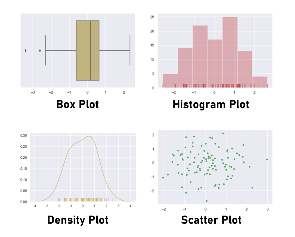
Here’s a code snippet to generate the previous plots:

import seaborn as sns
import numpy as np

# create two simple continious variables
x = np.random.normal(size=100)
y = np.random.normal(size=100)

# plot the distribution of the data
sns.distplot(x)

# create a density plot of x variable.
sns.distplot(x, hist=False, rug=True)

# creates a histogram plot of x variable with red color.
sns.distplot(x, kde=False, rug=True, color = "r");

# creates a box plot of x variable with green color.
sns.boxplot(x, color = "g");

# create a scatter plot of x and y variables.
sns.scatterplot(x, y, color = "g")

Discrete Variable

A discrete variable is a variable that can only take on a finite number of values, and these values are integers ( — which means numbers that are not a fraction), they are counts.

For example, the number of things bought by a customer in a supermarket is discrete. The customer can buy 2, 20, or 150 things, but not 10.4 items. It is always a round number.

The following are also examples of discrete variables:

Number of active bank accounts for a given client (1, 4, 7)
Number of pets in a family
The number of connected devices in a network

To visualize such discrete variables, you can use the following type of plots:

Count plot
Pie chart

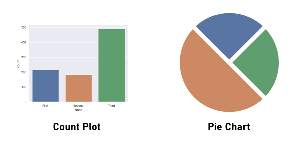
Here is a code snippet to obtain the previous plots:

import seaborn as sns
import matplotlib.pyplot as plt

# loading the titanic dataset.
titanic = sns.load_dataset("titanic")

# creating a count plot for the class variable.
sns.countplot(x="class", data=titanic)

# getting the count of each class
values = titanic["class"].value_counts().values

# getting the labels of each class.
labels = titanic["class"].value_counts().index

# creating the pie chart.
plt.pie(values, labels= labels,  shadow=True, startangle=90)

Categorical Variables

The values of a categorical variable are selected from a group of categories, also called labels. Examples are gender (male or female) and marital status (never married, married, divorced, or widowed).

Other examples of categorical variables include:

Gender (male, female)
Mobile network provider (Mobilis, Vodafone, Orange)
City name (Tiaret, Algiers, Texas, Dubai)

We can further categorize categorical variables into:

Ordinal variables
Nominal variables

Ordinal Variable

Ordinal variables are variables that exist within meaningfully ordered categories. For example:

Student grades on an exam (A, B, C, or F).
Days of the week (Sunday, Monday, Tuesday, …)

Nominal Variable

For nominal variables, there isn’t a natural order in the labels. For example, country of birth—with Algeria, USA, South Korea as values—is also categorical, but how they’re ordered doesn’t typically matter.

Other examples of nominal variables:

Car color (blue, grey, silver)
Car make(Citroen, Peugeot)
City (Tiaret, Cairo, Dubai)

There’s nothing that indicates a natural order of the labels, and in principle, they are all equal.

Dates and Times

A particular type of categorical variable are those that take dates or time as values.

For example:

Date of birth (16–04–1997, 12–01–2012)
Date of application (2020-Jan, 2022-Feb)

Datetime variables can contain dates only, time, or date and time.

We don’t usually work with datetime variables in their raw format because:

Date variables contain a considerable number of different categories
We can extract much more information from datetime variables by pre-processing them correctly.

Besides that, sometimes date variables contain dates that were not present in the dataset used to train the machine learning model. Similarly, date variables can also contain dates placed in the future, with respect to the dates in the training dataset.

Therefore, the machine learning model can’t understand what to do with these dates because it never saw them while being trained.

In ensuing posts, we’ll cover different techniques for engineering datetime variables.

Mixed Variables

Finally, mixed variables are those whose values can contain both numbers and labels.

For a variety of reasons, mixing variables can occur in a given dataset, especially when filling its values.

Consider this common example:

Let’s say we have a number of something, like the income, or the number of children.
Now let us say that this number could not be retrieved, for a variety of reasons, like we can’t income of a person because he committed to filling it when we did our survey to gather the data.
In this case, we can return a label, and this label can represent the reason behind the issue, like ERROR_OMMIT for client omit to answer.

So for some rows, this variable will hold a number that represents the income, and for others, the variable will contain the label ERROR_OMMIT, and that’s a mixed variable.

Conclusion

In this post, we discussed the different variable types you can find in a given dataset. We outlined the characteristics of each type and also saw how to visualize them with some pretty simple Python code.