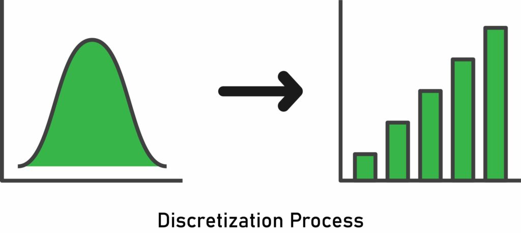
Hands-on with Feature Engineering Techniques: Variable Discretization

This article is all about variable discretization, which is the process of transforming a continuous variable into a discrete one. It essentially creates a set of contiguous intervals that span the variable’s value range.

Binning is another name for discretization, where the bin is an alternative name for the interval.

Discretization Approaches

There are multiple approaches to achieve this discretization. In this guide, we’ll explore the following methods:

Supervised Approach

Discretization with decision trees

Unsupervised Approaches

Equal-width discretization
Equal-frequency discretization
K-means discretization

Other

Custom discretization

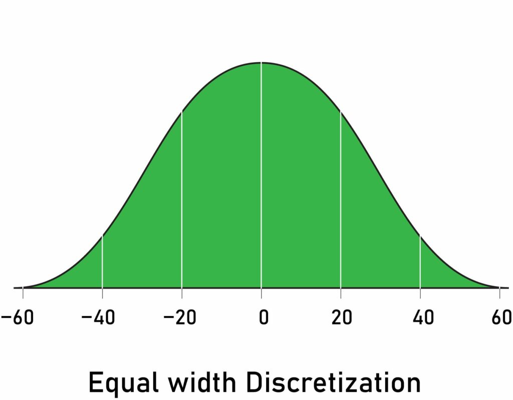
Equal-width Discretization

This is the most simple form of discretization—it divides the range of possible values into N bins of the same width.

The width of intervals is determined by the following formula:

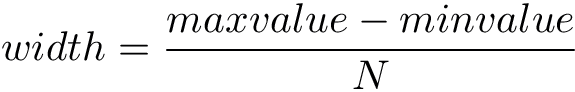
For example, if the variable interval is [100, 200], and we want to create 5 bins, that means 200-100 / 5 = 20, so each bin’s width is 20, and the intervals will be [100, 120], [120, 140],…,[180, 200].

When working with equal-width discretization, there are some points to consider:

Equal-width discretization does not improve the values spread.
This method handles outliers.
It creates a discrete variable (obviously).
It’s useful when combined with with categorical encodings.

Here is a code snippet in Python:

# import the libraries
import pandas as pd
from sklearn.preprocessing import KBinsDiscretizer

# load your data
data = pd.read_csv('yourData.csv')

# create the discretizer object with strategy uniform and 8 bins
discretizer = KBinsDiscretizer(n_bins=8, encode='ordinal', strategy='uniform') 

# fit the discretizer to the train set
discretizer.fit(train)

# apply the discretisation
train = discretizer.transform(train)
test = discretizer.transform(test)

Equal-Frequency Discretization

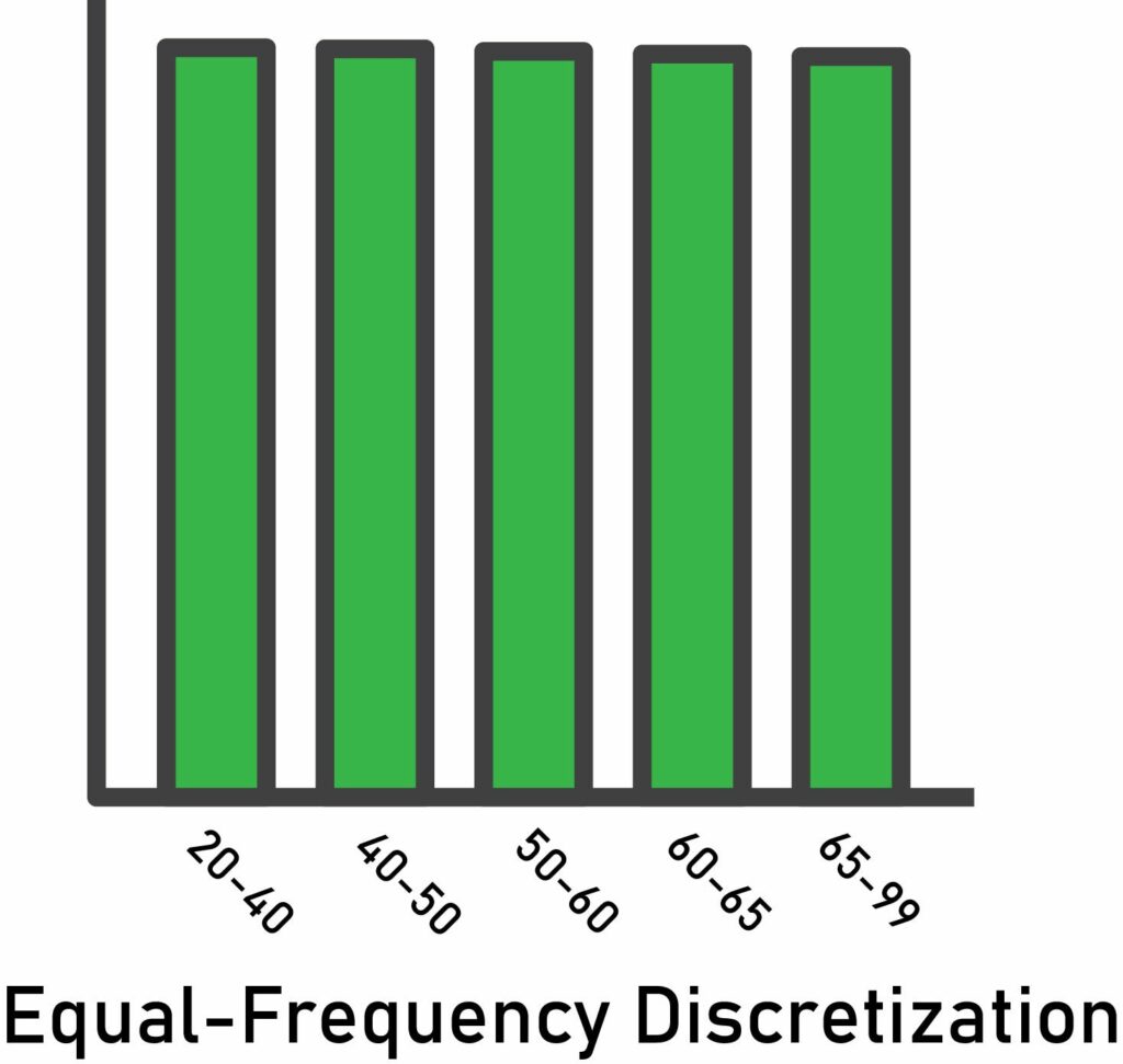
Equal-frequency discretization divides the scope of possible values of the variable into N bins, where each bin holds the same number (or approximately the same number) of observations.

When working with equal-frequency discretization, here are some points to consider:

In this method, the interval boundaries correspond to the quantiles.
This method improves the value spread.
Equal-frequency handles outliers.
This arbitrary binning may disturb the relationship with the target.
It’s useful when combined with with categorical encodings.

Here’s an illustration of the result of this method:

And a sample code snippet in Python:

# import the libraries
import pandas as pd
from sklearn.preprocessing import KBinsDiscretizer

# load your data
data = pd.read_csv('yourData.csv')

# create the discretizer object with strategy quantile and 8 bins
discretizer = KBinsDiscretizer(n_bins=8, encode='ordinal', strategy='quantile') 

# fit the discretizer to the train set
discretizer.fit(train)

# apply the discretisation
train = discretizer.transform(train)
test = discretizer.transform(test)

K-Means Discretization

This discretization method consists of applying k-means clustering to the continuous variable—then each cluster is considered as a bin.

First, let’s quickly review the k-means algorithm:

We create K random points. These points will be the center of clusters.
We associate every data point with the closest center (using some distance metric like Euclidean distance).
Finally, we re-compute each center position in the center of its associated points.

Here are some great tutorials about k-means:

When working with k-means methods, here are some points to consider:

This method does not improve the values spread.
It handles outliers, although outliers may influence the centroid.
It creates a discrete variable.
It’s useful when combined with with categorical encodings.

The code for this method is very simple—here’s the snippet:

# import the libraries
import pandas as pd
from sklearn.preprocessing import KBinsDiscretizer

# load your data
data = pd.read_csv('yourData.csv')

# create the discretizer object with strategy quantile and 8 bins
discretizer = KBinsDiscretizer(n_bins=6, encode='ordinal', strategy='kmeans') 

# fit the discretizer to the train set
discretizer.fit(train)

# apply the discretisation
train = discretizer.transform(train)
test = discretizer.transform(test)

Discretization with Decision Trees

Discretization with decision trees consists of using a decision tree to identify the optimal bins.

Technically, when a decision tree makes a decision, it assigns an observation to one of N end leaves. Accordingly, any decision tree will generate a discrete output, which its values are the predictions at each of its N leaves.

Steps for discretization with decision trees

First, we train a decision tree of limited depth (2, 3, or 4) using only the variable we want to discretize and the target.
Second, we replace the variable’s value with the output returned by the tree.

Here are some points to bear in mind:

It does not improve the values spread.
It handles outliers since trees are robust to outliers.
It creates a discrete variable.
It’s prone to over-fitting.
It costs some time to tune the parameters effectively (e.g., tree depth, the minimum number of samples in one partition, minimum information gain)
The observations within each bin are more similar to each other.
It creates a monotonic relationship.

Finally, here is the code with sklearn and Python:

# import the libraries
import pandas as pd
from sklearn.tree import DecisionTreeClassifier

# load your data
data = pd.read_csv('yourData.csv')

# create variables for the your target and the variable you want to discretize
x_variable = train['a_variable']
target = train['target']

# build the decision tree with max depth of your choice 
# {depth of 2 will create two splits, and 4 different bins for discretization}
decision_tree = DecisionTreeClassifier(max_depth=2)

# start the learning process.
decision_tree.fit(x_variable, target)

# apply the discretization to the variable.
train['a_variable'] = decision_tree.predict_proba(train['a_variable'].to_frame())[:, 1]
test['a_variable'] = decision_tree.predict_proba(test['a_variable'].to_frame())[:, 1]

Using the newly-created discreet variable

After the discretization process, what do we do with the results? In the previous code snippets, we used encode=’ordinal’, which results in integer encoding—basically, it assigns to the resulted interval/bins integer numbers like 1,2,3, etc.

There are two major methods to use these numbers in machine learning models:

We can use the value of the interval straight away if we decide to use intervals as numbers.
We can treat these numbers as categories; therefore, we can apply any of the encoding techniques that we’ve seen.
An advantageous way of encoding these bins when treating them as categories is to use an encoding technique that creates a monotone relationship with the target.

Custom Discretization

Oftentimes, when engineering variables in a custom environment (i.e. for a particular business use case), we determine the intervals in which we think the variable should be divided so that it makes sense for the business.

Typical examples are the discretization of variables like Age, we can divide it into groups like [0–10] as kids, [10–25] as teenagers (in other cases, we might adjust these ranges and associated labels), and so on.

Here’s a sample code snippet with Pandas to discretize the age variable:

# import the libraries
import pandas as pd

# bins interval
bins = [0, 10, 25, 65, 250]

# bins labels
labels = ['0-10', '10-25', '25-65', '>65']

# discretization with pandas
train['age'] = pd.cut(train.age, bins=bins, labels=labels, include_lowest=True)
test['age'] = pd.cut(test.age, bins=bins, labels=labels, include_lowest=True)

Conclusion

We saw in this post some methods to get started using discretization in your feature engineering process. Discretization can significantly improve classification performance. Many of the top contributions on Kaggle use discretization to create their machine learning models.

Editor’s Note: Heartbeat is a contributor-driven online publication and community dedicated to providing premier educational resources for data science, machine learning, and deep learning practitioners. We’re committed to supporting and inspiring developers and engineers from all walks of life.

Editorially independent, Heartbeat is sponsored and published by Comet, an MLOps platform that enables data scientists & ML teams to track, compare, explain, & optimize their experiments. We pay our contributors, and we don’t sell ads.

If you’d like to contribute, head on over to our call for contributors. You can also sign up to receive our weekly newsletters (Deep Learning Weekly and the Comet Newsletter), join us on Slack, and follow Comet on Twitter and LinkedIn for resources, events, and much more that will help you build better ML models, faster.