Evaluation Metrics for Machine Learning Models

Machine learning as a field is full of technical terms, making it difficult for beginners to get started. One might see things like “deep learning,” “the kernel trick,” “regularization,” “overfitting,” “semi-supervised learning,” “cross-validation,” etc. But what in the world do they mean?

One of the core tasks in building any machine learning model is to evaluate its performance. It’s fundamental, and it’s also really hard.

So how would one measure the success of a machine learning model? How would we know when to stop the training and evaluation and call it good? With this article, we’ll try to answer these questions. This article is organized as follows:

In the first section, we’ll introduce what we mean by “ML Model Evaluation” and why it’s actually necessary to evaluate any machine learning model. In subsequent sections, we’ll discuss various evaluation metrics available in relation to specific use cases in order to better understand these metrics.

1. Introduction

While data preparation and training a machine learning model is a key step in the machine learning pipeline, it’s equally important to measure the performance of this trained model. How well the model generalizes on the unseen data is what defines adaptive vs non-adaptive machine learning models.

By using different metrics for performance evaluation, we should be in a position to improve the overall predictive power of our model before we roll it out for production on unseen data.

Without doing a proper evaluation of the ML model using different metrics, and depending only on accuracy, can lead to a problem when the respective model is deployed on unseen data and can result in poor predictions.

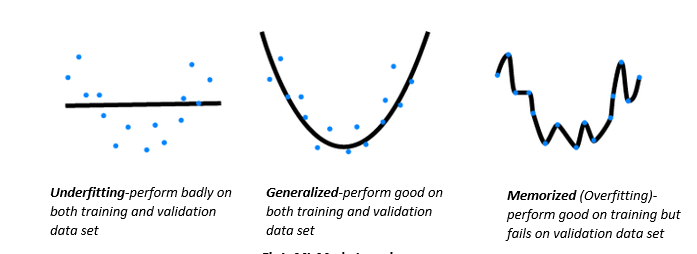
This happens because, in cases like these, our models don’t learn but instead memorize; hence, they cannot generalize well on unseen data. To get started, let’s define these three important terms:

Learning: ML model learning is concerned with the accurate prediction of future data, not necessarily the accurate prediction of training/available data.
Memorization: ML Model performance on limited data; in other words, overfitting on the known training dataset.
Generalization: Can be defined as the capability of the ML model to apply learning to previously unseen data. Without generalization there’s no learning, just memorization. But note that generalization is also goal specific —for instance, a well-trained image recognition model on zoo animal images may not generalize well on images of cars and buildings.

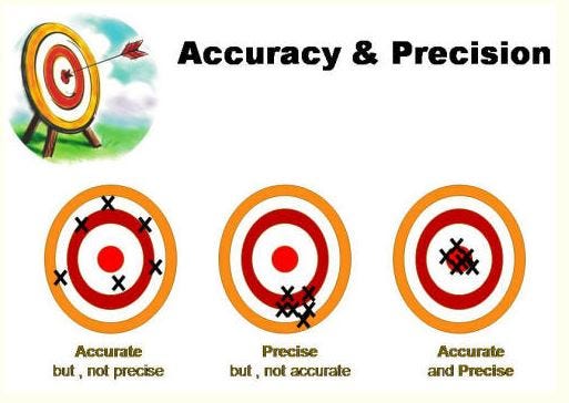
The images below depict how simply relying on model accuracy during training the model leads to poor performance during validation.

In the next section, we’ll discuss the different evaluation metrics available that could help in the generalization of the ML model.

2. Evaluation Metrics

Evaluation metrics are tied to machine learning tasks. There are different metrics for the tasks of classification, regression, ranking, clustering, topic modeling, etc. Some metrics, such as precision-recall, are useful for multiple tasks. Classification, regression, and ranking are examples of supervised learning, which constitutes a majority of machine learning applications.

2.1 Model Accuracy:

Model accuracy in terms of classification models can be defined as the ratio of correctly classified samples to the total number of samples:

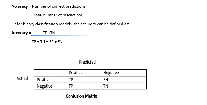
True Positive (TP) — A true positive is an outcome where the model correctly predicts the positive class.

True Negative (TN)—A true negative is an outcome where the model correctly predicts the negative class.

False Positive (FP)—A false positive is an outcome where the model incorrectly predicts the positive class.

False Negative (FN)—A false negative is an outcome where the model incorrectly predicts the negative class.

Though highly-accurate models are what we aim to achieve, accuracy alone may not be sufficient to ensure the model’s performance on unseen data. Let’s explore this with a couple of use cases:

Problem Statement– Build a prediction model for hospitals to identify whether the patient is suffering from cancer or not .

Binary Classification Model — Predict whether the patient has cancer or not.

Let’s assume we have a training dataset with labels—100 cases, 10 labeled as ‘Cancer’, 90 labeled as ‘Normal.’

Let’s try calculating the accuracy of this model on the above dataset, given the following results:

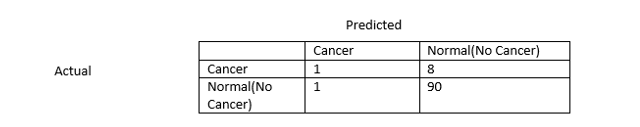
In the above case let’s define the TP, TN, FP, FN:

TP (Actual Cancer and predicted Cancer) = 1

TN (Actual Normal and predicted Normal) = 90

FN (Actual Cancer and predicted Normal) = 8

FP (Actual Normal and predicted Cancer) = 1

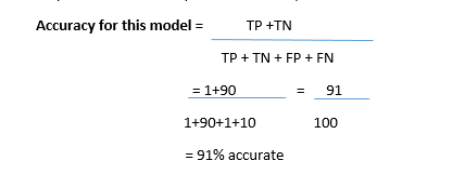
So the accuracy of this model is 91%. But the question remains as to whether this model is useful, even being so accurate?

This highly accurate model may not be useful, as it isn’t able to predict the actual cancer patients—hence, this can have worst consequences.

So for these types of scenarios how do we can trust the machine learning models?

Accuracy alone doesn’t tell the full story when we’re working with a class-imbalanced dataset like this one, where there’s a significant disparity between the number of positive and negative labels.

In the next section, we’ll look at two better metrics for evaluating class-imbalanced problems: precision and recall.

2.2 Precision and Recall

In a classification task, the precision for a class is the number of true positives (i.e. the number of items correctly labeled as belonging to the positive class) divided by the total number of elements labeled as belonging to the positive class (i.e. the sum of true positives and false positives, which are items incorrectly labeled as belonging to the class).

In this context, recall is defined as the number of true positives divided by the total number of elements that actually belong to the positive class (i.e. the sum of true positives and false negatives, which are items which were not labeled as belonging to the positive class but should have been).

Let’s try to measure precision and recall for our cancer prediction use case:

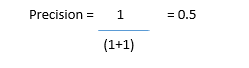
Our model has a precision value of 0.5 — in other words, when it predicts cancer, it’s correct 50% of the time.

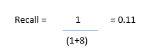
Our model has a recall value of 0.11 — in other words, it correctly identifies only 11% of all cancer patients.

Precision & Recall Tug-of-War:

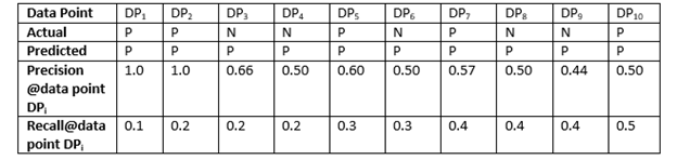
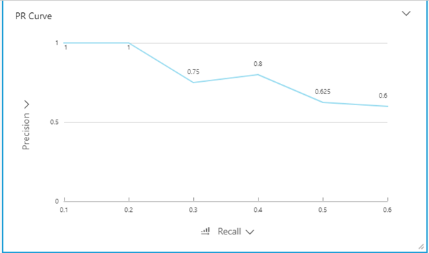
To fully evaluate the effectiveness of a model, it’s necessary to examine both precision and recall. Unfortunately, precision and recall are often in conflict. That is, improving precision typically reduces recall and vice versa. Let’s try to project this on PR (Precision-Recall) curve:

PR Curve:

Oftentimes, the domain use cases and costs associated with them determine whether high precision or high recall is most desirable. Let’s take a look at some examples of this:

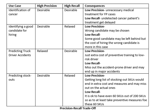
So whether high precision or high recall is preferred would depend upon the actual domain/use case, but there exists another evaluation metric known as an F1 Score that helps us get the best of both metrics.

2.3 F1 Score

The F1 score is the harmonic mean of the precision and recall, where an F1 score reaches its best value at 1 (perfect precision and recall) and worst at 0.

Why harmonic mean? Since the harmonic mean of a list of numbers skews strongly toward the least elements of the list, it tends (compared to the arithmetic mean) to mitigate the impact of large outliers and aggravate the impact of small ones:

An F1 score punishes extreme values more. Ideally, an F1 Score could be an effective evaluation metric in the following classification scenarios:

When FP and FN are equally costly—meaning they miss on true positives or find false positives— both impact the model almost the same way, as in our cancer detection classification example
Adding more data doesn’t effectively change the outcome effectively
TN is high (like with flood predictions, cancer predictions, etc.)

2.3 ROC Curve

A receiver operating characteristic curve, or ROC curve, is a graphical plot that illustrates the diagnostic ability of a binary classifier system as its discrimination threshold is varied.

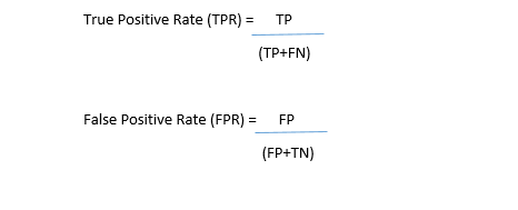
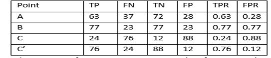
The ROC curve is created by plotting the true positive rate (TPR) against the false positive rate (FPR) at various threshold settings. The true positive rate is also known as sensitivity, recall, or probability of detection in machine learning. The false-positive rate is also known as the fall-out, or probability of false alarm.

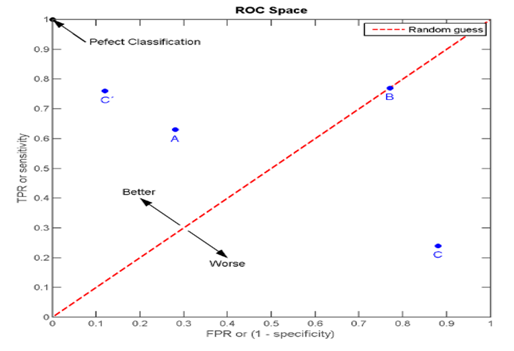
Points A, B, C, and C’ represent the graph locations at different TPR and FPR, as illustrated in the below table:

Point (0,0)– represents the strategy of never issuing a positive classification; such a classifier commits no false positive errors but also gains no true positives.

Point(1,1)- represents the strategy of always issuing a positive classification; such a classifier gets all positives, but the false positive rate would also be very high.

So the best possible prediction model would yield a point in the upper left corner or coordinate (0,1) of the ROC space, representing 100% sensitivity (no false negatives) and 100% specificity (no false positives). The (0,1) point is also called a Perfect Classification.

A random guess would give a point along a diagonal line (the so-called line of no-discrimination) from the left bottom to the top right corners (regardless of the positive and negative base rates).

ROC curves have an attractive property: they are insensitive to changes in class distribution. If the proportion of positive to negative instances changes in a test set, the ROC curves won’t change. This feature of ROC curve is known as Class skew independence.

This is because the metrics TPR and FPR used for ROC are independent of the class distribution as compared to other metrics like accuracy, precision, etc., which are impacted by imbalanced class distributions.

But how do we compute the points in an ROC curve? We could evaluate a logistic regression model many times with different classification thresholds, but this would be inefficient. Fortunately, there’s an efficient, sorting-based algorithm that can provide this information for us, called AUC.

2.4 AUC — Area under the ROC Curve

An ROC curve is a two-dimensional depiction of classifier performance. To compare classifiers, we may want to reduce ROC performance to a single scalar value representing expected performance. A common method is to calculate the area under the ROC curve, abbreviated AUC.

Since the AUC is a portion of the area of the unit square, its value will always be between 0 and 1.0. However, because random guessing produces the diagonal line between (0, 0) and (1, 1), which has an area of 0.5, no realistic classifier should have an AUC less than 0.5

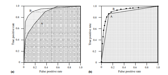
Fig. 4a shows the areas under two ROC curves, A and B. Classifier B has greater area and therefore better average performance. Fig. 4b shows the area under the curve of a binary classifier A and a scoring classifier B.

It’s possible for a high-AUC classifier to perform worse in a specific region of ROC space than a low-AUC classifier. Fig. 4a shows an example of this: classifier B is generally better than A except at FP rate > 0.6, where A has a slight advantage. But in practice, AUC performs very well and is often used when a general measure of prediction is desired.

AUC is desirable for the following two reasons:

AUC is scale-invariant. It measures how well predictions are ranked, rather than their absolute values.
AUC is a classification-threshold-invariant. It measures the quality of the model’s predictions irrespective of what classification threshold is chosen.

2.5 Multi-Class ROC

With more than two classes, classifications problem become much more complex if the entire space is to be managed. With n classes, the confusion matrix becomes an n · n matrix containing the n correct classifications (the major diagonal entries) and n*n — n possible errors (the off-diagonal entries). Instead of managing trade-offs between TP and FP, we have n benefits and n*n — n errors. With only three classes, the surface becomes a 3*3- 3 = 6-dimensional polytope.

One method for handling n classes is to produce n different ROC graphs, one for each class.

Specifically, if C is the set of all classes, ROC graph i plots the classification performance using class ci as the positive class and all other classes as the negative class:

Pi = Ci

Ni = Union(Cj) for j≠i

Multi-Class AUC: Similarly, AUC can be calculated for multi-class problems by generating each class reference ROC curve in turn, measuring the area under the curve and then summing the AUCs weighted by the reference class’s prevalence in the data.

3. Conclusion

Understanding how well a machine learning model is going to perform on unseen data is the ultimate purpose behind working with these evaluation metrics. Metrics like accuracy, precision, recall are good ways to evaluate classification models for balanced datasets, but if the data is imbalanced and there’s class disparity, then other methods like ROC/AUC perform better in evaluating the model performance.

As we’ve seen, the ROC curve isn’t just a single number; it’s a whole curve. It provides nuanced details about the behavior of the classifier, but it’s also hard to quickly compare many ROC curves to each other. The AUC is one way to summarize the ROC curve into a single number so that it can be compared easily and automatically. A good ROC curve has a lot of space under it (because the true positive rate shoots up to 100% very quickly). A bad ROC curve covers very little area. So high AUC is good, and low AUC is not so good.

One last important point to keep in mind, since we focused largely on classification tasks in this guide: Any machine learning model should be optimized and evaluated according to the task it’s built to address.