
In the last article, we discussed 3 general and common situations faced when handling data: optimizing how to read CSV files with a lot of unnecessary columns, using the map method to create new category columns, and finding empty strings in your DataFrame that aren’t labeled as null.
However, another common characteristic of real-life data is the presence of missing values—in other words, an incomplete dataset. If you’ve worked with real-life data before, you can understand how frustrating it can be working with missing values, especially if the data is going to be used to train a model. This is because most of the existing machine learning models don’t work well with missing values.
What causes missing data values?
The causes of missing values can be categorized into two primary types:
A. Value missing at random
B. Value missing, but not at random
A. Value missing at random
This is when the chances of any value in that feature being missing are the same. Or in other words, the value missing has nothing to do with the observation being studied. For example—when a piece of information during processing is lost or misplaced regardless and independent on any other information been observed as well.
B. Value missing, but not at random
This is when the chances of any value in that feature being missing are not the same. Or in other words, the values missing are dependent on a certain feature being observed in the dataset. For example—when both genders are being inquired about their weight or age, there may be a higher probability that there will be more females with missing values than males. This could be as a result of withholding information that is too sensitive for one sex.
But how can we fix these missing values? This is what’s called imputation in statistics.
There are quite a few imputation methods. However, when deciding what method to use, there are some things to keep in mind. We can frame these concerns by asking 3 questions:
- What is the type of the variable (data type) of the feature?
- How does the imputation method affect the distribution of the data?
- What is the cause of the missing value?
Data type
Data types can be identified commonly as Numerical and Categorical. These data types affect what method we should use. For example, it wouldn’t be wise to replace a categorical variable with the mean of the variables or replace a numerical variable with a categorical method.
Data distribution
There are different types of data distributions, but we’ll focus on the common ones: normal distribution and skewed distribution (be it right-skewed or left-skewed). An imputation method could distort the distribution, and this could reduce the performance of a linear machine learning model. However, the degree of distortion depends greatly on the percentage of missing values imputed.
Dataset Overview
For the purpose sof this article, a hypothetical dataset was generated that consists of 5 columns (City, Degree, Age, Salary, Marital Status) and 10 rows. Let’s assume each row is an entry of participants’ details on a survey. And assume that our aim is to predict if a person is married or not based on the other feature/ columns available.

Let jump into the types of imputation methods
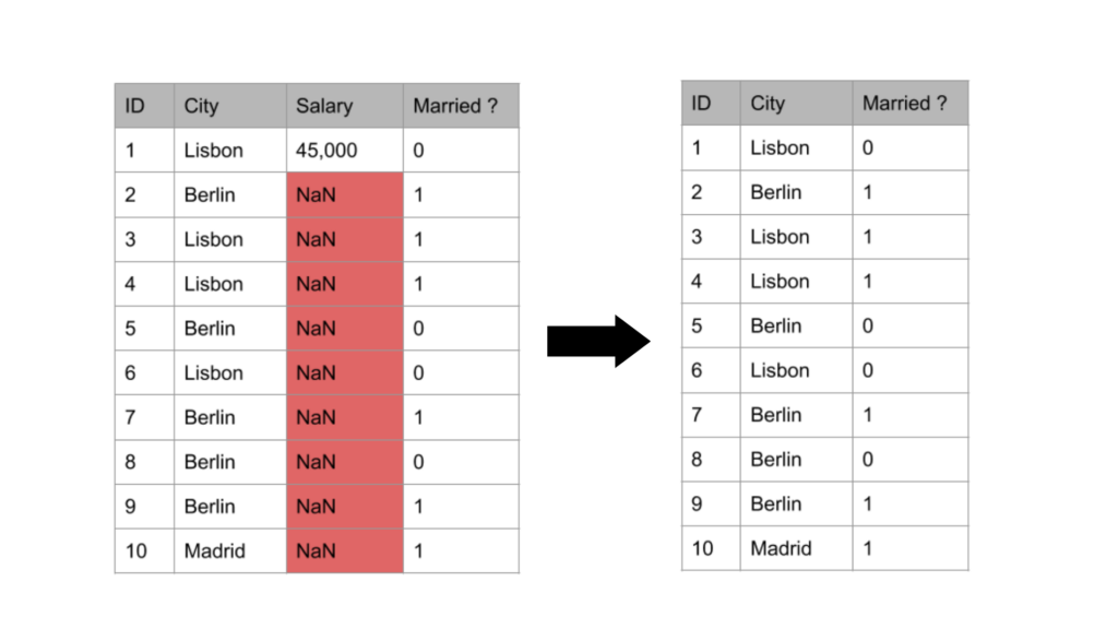
1. Complete removal of rows or columns of missing values
This is one of the most intuitive and simple methods. As it implies, it includes removing all rows or columns that have missing values present. This method can be used regardless of the variable’s nature as numerical or categorical.
Removal of rows

From the above diagrams, we see that after removing the rows with missing values, the number of rows reduced from 10 to 6, removing all the other non-missing values, along with the missing values
Removal of columns
From the above diagram, we see that the number of columns reduced from 3 to 2
This method makes more sense to use when the values are missing at random (i.e no dependency between that feature and any other feature in the dataset). There are two advantages to this method:
- No data manipulation is required
- It preserves variable distribution
As intuitive as it may be, it’s a method that needs to be used with caution.
- This is because the removal of rows and columns could mean losing important information about the data along with the missing values.
- Another reason is that when using your model in production, the model will not automatically know how to handle missing data.
A couple rules of thumb to follow when using this method:
- Rows of missing values can be removed when the NULL values (missing values) are around 5% (or less) of the total data.
- Columns of missing values can be completely removed when the NULL values are significantly more than the other values present. In this situation, it wouldn’t make sense to keep these columns, as they hold little or no descriptive information about the data.
2. Mean/Median & Mode Imputation
This method involves replacing the missing value with a measure of central tendency of the column it’s present in. These measures are mean and median if the column variable type is numerical, and mode if the column variable type is categorical.
For numerical variables
Mean as a measure is greatly affected by outliers or if the distribution of the data or column is not normally-distributed. Therefore, it’s wise to first check the distribution of the column before deciding if to use a mean imputation or median imputation
Using our example dataset, let’s see what the result of this method will look like:

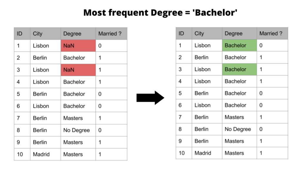
For categorical variables
Mode imputation means replacing missing values by the mode, or the most frequent- category value.
The results of this imputation will look like this:
It’s good to know that the above imputation methods (i.e the measures of central tendency) work best if the missing values are missing at random. In these cases, it can be fair to assume that the missing values are most likely very close to the value of the mean, median, or mode of the distribution, as these represent the most frequent/average observations.
There are two advantages to this method:
- It’s easy to implement
- This method can be integrated into production or for a future unknown dataset
However, there are some downsides:
- It distorts the distribution of the dataset
- It distorts the variance of the dataset by reducing the variance; i.e. the new variance is underestimated compared to the original variance before imputing. This is because this method creates similar values in the distribution, which shortens the interquartile range and in turn creates more outliers.
- It also distorts the co-variance, i.e. the relationship of that feature with other features in the dataset.
- In the case of categorical variables, mode imputation distorts the relation of the most frequent label with other variables within the dataset and may lead to an over-representation of the most frequent label if the missing values are quite large.
Because of all these disadvantages, it’s recommended to use this method when the missing values are around 5% (or less) of the total data
3. Systematic Random Sampling Imputation
This method involves substituting the missing values with values extracted from the original variable. It can be applied to both numerical and categorical variables. It’s also used when the values are missing at random.
The idea here is to replace the population of missing values with a population of the original variables with the same distribution. Therefore, the variance and distribution of the variable are preserved.
But why systematic and not completely random? This is because we want to be able to reproduce the same value every time the variable is used. And how? By specifying a random state.
The results of this imputer will look like this:

From the above example, our imputer randomly chooses 30 and 25, which are the most frequent values. This make intuitive sense because values that are more frequent are more likely to be selected than values that are less frequent. In a sense, it’s like using a mode imputer without distorting the distribution of the variable.
Some advantages this method has over the mean/median/mode imputation include:
- It does not distort the variance
- It does not distort the distribution, regardless of the percentage of missing values replaced
- Because of the above reason, it could be better suited for linear models
However, it does have a couple of serious downsides to consider:
- Although it has a clear advantage over the mean/median imputation method, it isn’t widely used, comparatively. This could be because of the element of randomness.
- When replacing missing values in the test set as well, the imputed values from the train set will need to be stored in memory.
Other methods to use, especially if the values are not missing at random
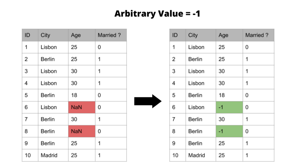
4. Arbitrary values imputation
This involves using an arbitrary value to replace the missing values. One can think of them as placeholders for the missing values. This is a method used for numerical variables.
The most commonly used numbers for this method are -1, 0,99, -999 (or other combinations of 9s). Deciding on which arbitrary number to use depends on the range of your data’s distribution. For example, if your data is between 1–100, it wouldn’t be wise to use 1 or 99 because those values may already exist in your data, and these placeholder numbers are usually used to flag missing values.
The result of this imputer will look like this
It’s good to know that the advantages and the disadvantages of this method are similar to the mean/median and mode method. However, instead of underestimating the variance, it overestimates the variable by expanding the spread or range.
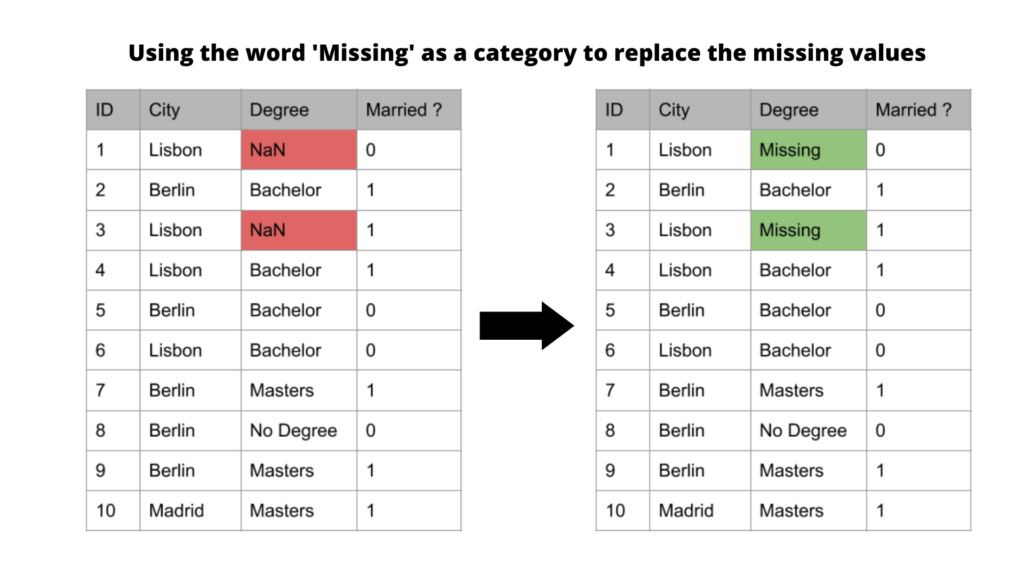
5. Missing Category Imputation
This method is used for categorical data. It involves labeling all missing values in a categorical column as ‘missing’.
The result of this imputer will look like this:
The advantage this method has over the other methods discussed is that it makes no assumption about the missing values (i.e be it random or not random or replacing the missing value with an estimate). However, it’s good to point out that this method creates an additional cardinality for your column. Therefore, it doesn’t work well for small amounts of missing values, as it creates rare labels that may lead to overfitting.
6. Missing Indicator Imputation
This method can be used for both numerical and categorical variables. The missing indicator method creates an additional binary variable that indicates whether the data was missing for observation or not (i.e 1 as missing and 0 as not missing).
This method is typically used in combination with other imputation methods, and especially methods that assume the value is missing at random(except the complete removal method, for good reasons). The creation of a binary missing indicator assumes that the missing values are predictive.
The result of this imputer will look like this:

As we can see from the above diagram, the number of columns has increased from 3 to 4, and the missing values were replaced by the mode of the column/variable.
There are some added complications to this method:
- It expands feature space and dimensionality—i.e if the dataset contains 20 features, and all of them have missing values, after adding a missing indicator for each column, we end up with a dataset of 40 features
- The original variable will still need to be imputed to remove the NULL values.
- It may lead to multi-collinearity between the original column and the new column and may reduce the performance of a linear model.
Conclusion
As you may have perceived, deciding what imputation method to use means deciding how much distribution distortion your model can perform well with. It also depends on what data type you want to replace and the cause of the missing values.
However, missing values are not the only characteristics of real-life data. Another common characteristic is dealing with categorical data for machine learning models. This is also known as categorical encoding. This is what we’ll be discussing in the next post in this series. So stay tuned.
Comments 0 Responses