
Deep neural networks perform incredibly well on computer vision tasks such as classification, object detection, and segmentation, but what do they consider before performing these tasks, and what does it take to make these decisions?
Interpreting neural network decision-making is an ongoing area of research, and it’s quite an important concept to understand. Neural networks are used in the real-world, so we can’t treat them like black boxes—we need to learn what they interpret, how they interpret, and what information each layer/channel in a neural network has learned.
For example if a self-driving car makes a bad decision and kills a person, if we aren’t able to quantify the reason for this bad decision, then we won’t be able to rectify it, which could lead to even more disasters.
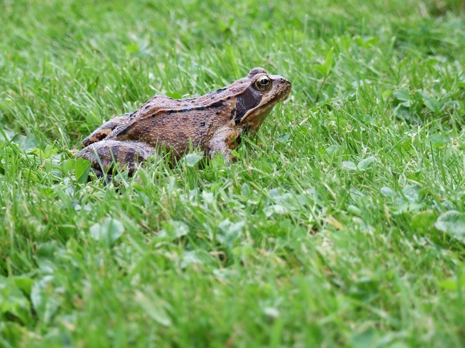
Consider the above image. We’d like a classification neural network to classify it as a frog. If our training data includes images that are similar to the one above (i.e. a frog crouched in grass), then what will happen when suddenly in our test set we encounter an image such as the one below?
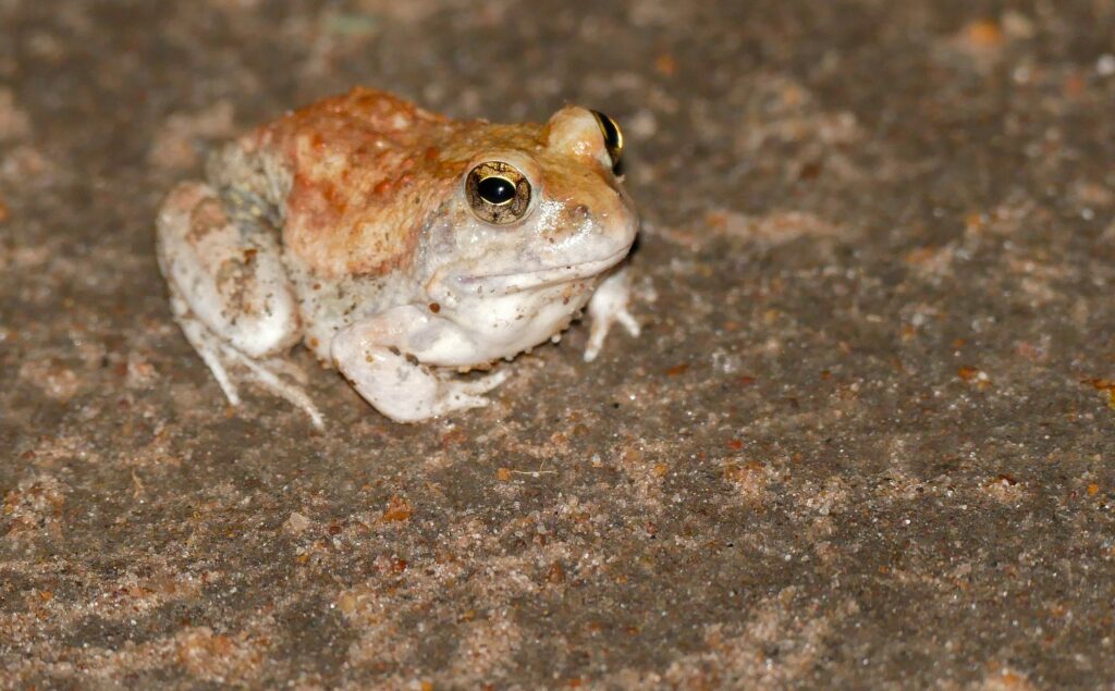
There’s a high probability that the network will fail—the network has looked at a lot of images with frogs in grass during training and has likely put too much emphasis on the background grass features rather than the frog features.
But without actually understanding what’s happening inside our neural network, we remain unaware of all this. We don’t know where the network is looking and what it’s concentrating on, or what features it’s relying on while making a decision. Thus, visualizing neural networks is absolutely essential in making them work robustly in practical, real-world use cases.
In this guide, we’ll discuss a few approaches such as activation maximization, occlusion-based heatmaps, and class activation mapping, which can be use to interpret what neural networks are looking for in images while making a decision.We’ll also discuss class activation mapping in detail and its upgrades Gradcam and Gradcam++, including how it can improve our understanding of neural network decisions.
Activation Maximization
In general when you consider the training of a neural network, weights at every layer are updated while the input is fixed, such that the prediction error is minimized. What if we slightly modify the above? What if we fix the weights of the entire network and try to update the input image (i.e the pixels present in the input image) such that activation at a particular layer is maximized.
What we get is activation maximization. What we’re trying to do with this technique is see what kind of input maximally activates a layer. This tells us what kind of information a particular layer is trying to capture and hence getting activated/lit up when certain input is passed.
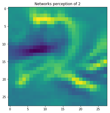
For example, below we have the input image generated by following the above procedure on the MNIST dataset, and it clearly depicts that this particular neuron gets activated when an image in line number 2 is passed as an input.
Occlusion-based heatmaps
Occlusion-based heatmaps attempt to determine all the important regions in an image that the neural network pays attention to while doing a task such as classification.
To achieve this, a patch of an image, such as the brown patch shown below, is slid over the image from top-left to bottom-right, just like we’d do in the case of object detection using a sliding window.
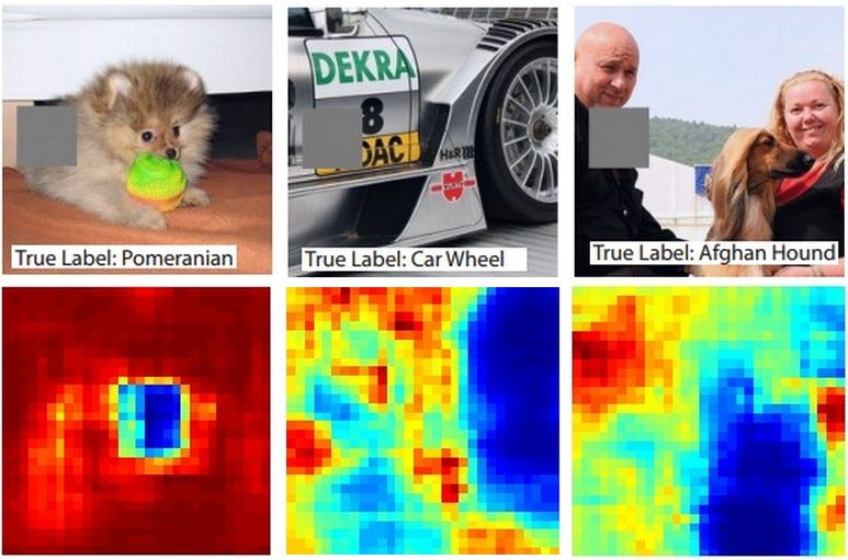
As we slide the patch across the region, we calculate the probability of predictions at each position of the patch. A heatmap of the image is then generated using these probability values. The heatmap signifies which parts of the image are more important.
If we look at the above image of the dog, we can see that (very probably) the face of the dog is quite important for the network to classify the image as a dog—hence, more value in the heatmap.
The problem with this kind of approach is that the box size is unknown and the process takes a lot of time, since the patch has to be moved across the entirety of the image. Additionally, the image has to be run through the network every time, leading to an unnecessary increase in required computational resources.
Class Activation Mapping
A recent study on using a global average pooling (GAP) layer at the end of neural networks instead of a fully-connected layer showed that using GAP resulted in excellent localization, which gives us an idea about where neural networks pay attention.
Even though the model in this case was trained for classification, by looking at the areas where the network paid attention, this method achieved decent results in object localization (i.e drawing a bounding box around the object), even though the network was never trained for that task. This was done by generating a heatmap of attention, similar to the one we saw in occlusion-based method above.
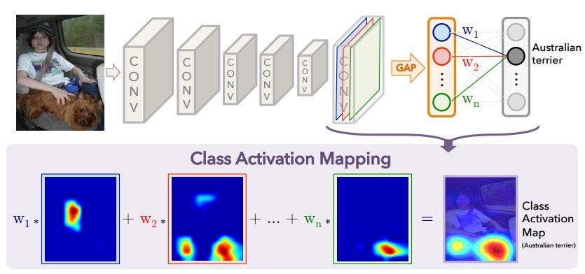
Now let’s discuss the approach through which we can achieve this visualization. For making class activation mapping (CAM) work, we need the network to be trained with a GAP layer. After that layer, we maintain a fully-connected network followed by a softmax layer, providing a class such as Australian terrier, shown above. Now if we want to generate the heatmap of Australian terrier in the image, we follow the below steps:
- Get all the weights connected between the fully-connected layer and the softmax class for which we want to predict—i.e weights w1, w2, …. wn, as shown in above figure. So if n feature maps are present before the GAP layer, we’ll get n weights connecting between the fully-connected layer and the softmax layer.
- Next we take the feature maps that are about to be passed through GAP layer. There are n feature maps, as we saw in the previous step. We multiply each feature map serially with a weight and add them (as shown above). Each weight tells us how much importance needs to be given to every individual channel in the entire feature map. The final weighted sum gives us a heatmap of a particular class (in this case, the Australian terrier). The heatmap size is the size of the feature map. To impose it on the input image, we scale it to the size of the input image and then overlay it on top of the input to get a result like the one above.
Limitations of CAM:
- Need to have a GAP layer in architecture. If not, we can’t apply this method.
- Can only be applied to visualize the final layer heatmap—can’t be used if we wanted to visualize a previous layer in the network.
These limitations are addressed in an improvement to this method: Grad-CAM
Gradient Weighted Class Activation Mapping (Grad-CAM)
To address the above issues, Grad-CAM is proposed, which has no restrictions in terms of using GAP, and can create heatmaps by visualizing any layer in the network. Let’s explore how this is achieved.
We have seen above that in CAM we generate heatmaps by taking the weighted average of layer output channels using the weights of the fully-connected network that’s connected to the output class.
In Grad-CAM, we do something similar, the only difference being the way in which these weights are generated. The gradient of the output class value with regards to each channel in the feature map of a certain layer is calculated. This results in a gradient channel map with each channel in it representing the gradient of the corresponding channel in a feature map.
The gradient channel map obtained is then global average pooled, and the values obtained henceforth are the weights of importance of each channel in the feature map. The weighted feature map is then used as a heatmap, just like in CAM. Since the gradient output can be calculated with regards to any layer, there’s no restriction of only using a final layer—also there’s no mention of network architecture anywhere, so any kind of architecture works.
Keras code to generate heatmap with Grad-CAM
The entire source code is available here:
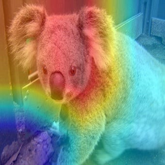
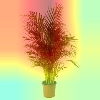
Below are some of the results that are achieved by generating heatmaps using Grad-CAM. As we can see, the main object is being focused on by the network, and hence the network is performing well.
Below is a cool representation of what the network concentrates on as we move from its initial layers to its final layers. In this case, the target output is glasses, and we can see that the initial layers aren’t concentrating exactly on the glasses, but we can also see that as we reach the final layers, they’re able to focus on the sunglasses.
As we can see from above Grad-CAM outputs are quite appealing and would definitely help a human in better understanding a neural network and in working along with it.
There is one limitation with Grad-CAM, though. If there’s more than one instance of a single class present in the image—for example if there are multiple cats present in an image for a cats vs dogs classifier—Grad-CAM won’t be able to identify all the instances of the class. This is solved using Grad-CAM++
The major update in Grad-CAM++ is during computing the GAP of the gradient channel map, only the positive values are considered and the negative values are ignored.
This is achieved by using a RELU on top of each value of the gradient channel map output. This approach of ignoring the negative gradients is commonly used in guided backpropagation.
The main reason for using only positive gradients is that we want to know which pixels have a positive impact on the class output—we don’t care which pixels have a negative impact. Also, if we don’t neglect the negative gradient, the negative values cancel few of the positive values in the gradient channel map while performing global average pooling. As a result, we lose valuable information, which can be avoided by neglecting negative gradients.
GradCAM Source: https://arxiv.org/pdf/1610.02391.pdf
GradCAM++ Source: https://arxiv.org/pdf/1710.11063.pdf
Conclusion
We have taken a tour of various algorithms for visualizing neural network decision-making, with an emphasis on class activation maps. Neural network result interpretation is an often ignored step, but as we have seen, it can help greatly in improving the results if utilized properly.
In the example we discussed above, if we can visualize and observe that the background of the frog is the reason for the failure of the network, we can improve our training dataset by adding more frog images with different backgrounds. Thus, we can achieve better results with the help of visualization techniques.
Further Reading: We have seen how individual neurons/channels/layers can impact the decision-making of a network. But there are many cases where a combination of these work to perform a decision, and hence, they might make more sense to be viewed together.

Comments 0 Responses