
Computer-based processing and identification of human voices is known as speech recognition. It can be used to authenticate users in certain systems, as well as provide instructions to smart devices like the Google Assistant, Siri or Cortana.
Essentially, it works by storing a human voice and training an automatic speech recognition system to recognize vocabulary and speech patterns in that voice. In this article, we’ll look at a couple of papers aimed at solving this problem with machine and deep learning.
Deep Speech 1: Scaling up end-to-end Speech Recognition
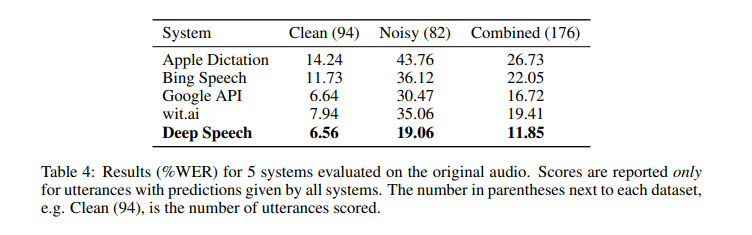
The authors of this paper are from Baidu Research’s Silicon Valley AI Lab. Deep Speech 1 doesn’t require a phoneme dictionary, but it uses a well-optimized RNN training system that employs multiple GPUs. The model achieves a 16% error on the Switchboard 2000 Hub5 dataset. GPUs are used because the model is trained using thousands of hours of data. The model has also been built to effectively handle noisy environments.
The major building block of Deep Speech is a recurrent neural network that has been trained to ingest speech spectrograms and generate English text transcriptions. The purpose of the RNN is to convert an input sequence into a sequence of character probabilities for the transcription.
The RNN has five layers of hidden units, with the first three layers not being recurrent. At each time step, the non-recurrent layers work on independent data. The fourth layer is a bi-directional recurrent layer with two sets of hidden units. One set has forward recurrence while the other has backward recurrence. After prediction, Connectionist Temporal Classification (CTC) loss is computed to measure the prediction error. Training is done using Nesterov’s Accelerated gradient method.
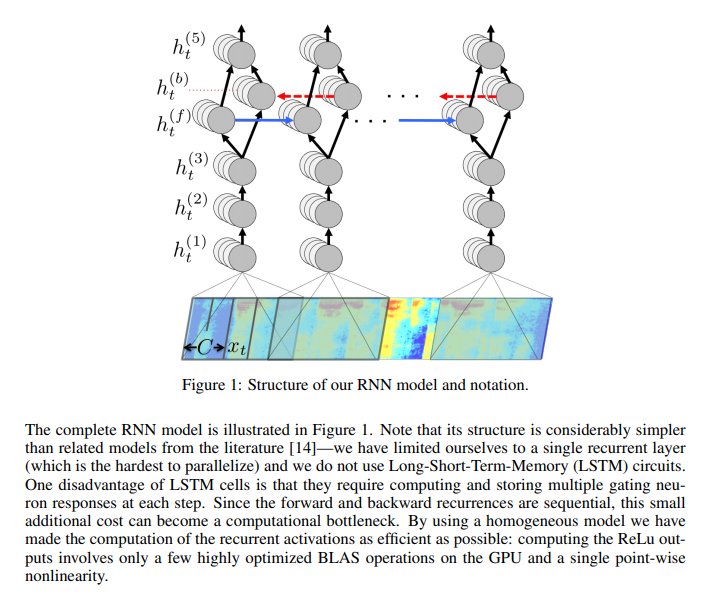
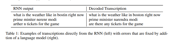
In order to reduce variance during training, the authors add a dropout of between 5% and 10% in the feedforward layers. However, this isn’t applied to the recurrent hidden activations. They also integrate an N-gram language model in their system because N-gram models are easily trained from huge unlabeled text corpora. The figure below shows an example of transcriptions from the RNN.
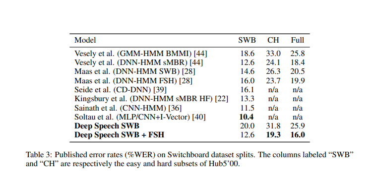
Here’s how this model performs in comparison to other models:
Deep Speech 2: End-to-End Speech Recognition in English and Mandarin
In the second iteration of Deep Speech, the authors use an end-to-end deep learning method to recognize Mandarin Chinese and English speech. The proposed model is able to handle different languages and accents, as well as noisy environments. The authors use high-performance computing (HPC) techniques to achieve a 7x speed increment from their previous model. In their data center, they implement Batch Dispatch with GPUs.
The English speech system is trained on 11,940 hours of speech, while the Mandarin system is trained on 9,400 hours. During training, the authors use data synthesis to augment the data.
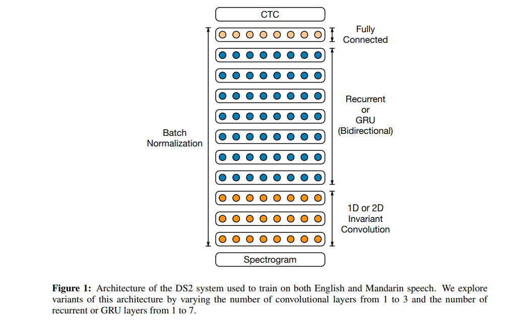
The architecture used in this model has up to 11 layers made up of bidirectional recurrent layers and convolutional layers. The computation power of this model is 8x faster than that of Deep Speech 1. The authors use Batch Normalization for optimization.
For the activation function, they use the clipped rectified linear (ReLU) function. At its core, this architecture is similar to Deep Speech 1. The architecture is a recurrent neural network trained to ingest speech spectrograms and output text transcriptions. The model is trained using the CTC loss function.
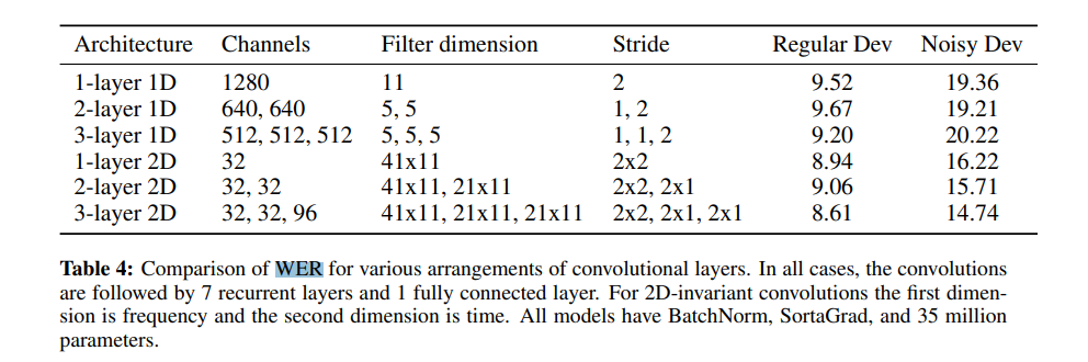
Below is a comparison of the Word Error Rate comparison for various arrangements of convolution layers.
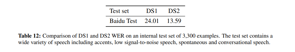
The comparison of the Word Error Rate of Deep Speech 1 and Deep Speech two is shown below. Deep Speech 2 has a much lower Word Error Rate.
The authors benchmark the system on two test datasets from the Wall Street Journal corpus of news articles. The model outperforms humans on the Word Error Rate on three out of four occasions. The LibriSpeech corpus is also used.
First-Pass Large Vocabulary Continuous Speech Recognition using Bi-Directional Recurrent DNNs
The authors of this paper are from Stanford University. In this paper, they present a technique that performs first-pass large vocabulary speech recognition using a language model and a neural network.
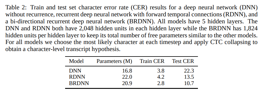
The neural network is trained using the connectionist temporal classification (CTC) loss function. CTC enabled the authors to train a neural network that predicts the character sequence of test utterances on the Wall Street Journal LVCSR corpus with a character error rate (CER) below 10%.
They integrate an n-gram language model with the CTC trained neural networks. The architecture of this model is Reaction-diffusion neural networks (RDNN). A modified version of the rectifier nonlinearity that clips large activations to prevent divergence during network training is used. Here are the character error rates results obtained by the RDNN.
English Conversational Telephone Speech Recognition by Humans and Machines
Authors from IBM Research present this paper aimed at verifying whether speech recognition techniques have achieved human performance. They also present a set of acoustic and language modeling techniques.
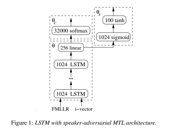
The acoustic side has three models: one LSTM with multiple feature inputs, a second LSTM trained with speaker-adversarial multitask learning, and a third residual net with 25 convolutional layers.
The language model uses character LSTMs and convolutional WaveNet-Style language models. The authors’ English conversational telephone LVCSR system has a Word Error Rate of 5.5%/10.3% on the Switchboard/CallHome subsets (SWB/CH).
The architecture used in this paper consists of 4–6 bidirectional layers with 1024 cells per layer, one linear bottleneck layer with 256 units, and an output layers with 32K units. Training consists of 14 passes of cross-entropy followed by 1 pass of Stochastic Gradient Descent (SGD) sequence training using the boosted MMI (Maximum Mutual Information) criterion.
This process is smoothed by adding the scaled gradient of cross-entropy loss. The LSTM was implemented in Torch with CuDNN version 5.0 backend. Cross-entropy training for each model was done on a single Nvidia K80 GPU device and took about two weeks for 700M samples per epoch.
For the convolutional network acoustic modeling, the authors trained residual networks. The next table shows several ResNet architectures and their performance on the test data.
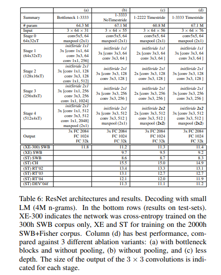
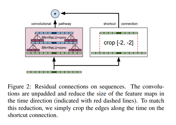
The figure below shows how the residual networks were adapted for acoustic modeling. The network has 12 residual blocks, 30 weight layers, and 67.1M parameters. Training was done using the Nesterov accelerated gradient with learning rate 0.03 and momentum 0.99. The CNN was also implemented on Torch using the cuDNN v5.0 backend. The cross-entropy training took 80 days for 1.5 billion samples using a Nvidia K80 GPU with a 64 batch size per GPU.
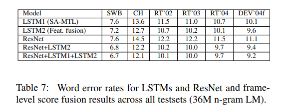
Let’s now look at the word error rates for the LSTMs and ResNets:
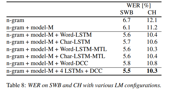
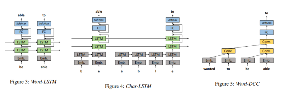
The authors also experimented with four LSTM language models, namely WordLSTM, Char-LSTM, Word-LSTM-MTL, and Char-LSTM-MTL. The figure below shows their architecture.
The Word-LSTM has one word-embedding layer, two LSTM layers, one fully-connected layer, and one softmax layer. The Char-LSTM has an LSTM layer to estimate word embeddings from character sequences. Both Word-LSTM and Char-LSTM used cross-entropy loss for predicting the next word. Multi-task learning (MTL) is introduced in Word-LSTM-MTL and Char-LSTM-MTL.
WordDCC consists of a word embeddings layer, causal convolution layers with dilation, convolution layers, fully-connected layers, a softmax layer, and residual connections.
Wav2Letter++: The Fastest Open-source Speech Recognition System
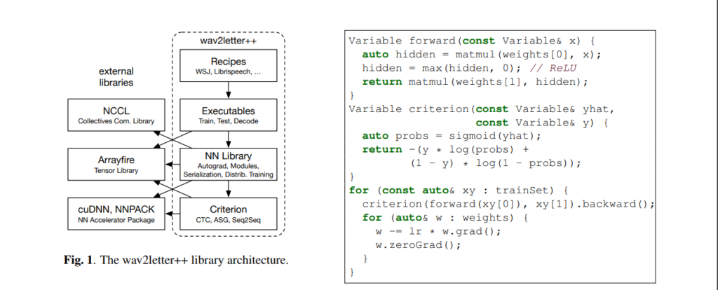
Authors from Facebook AI Research propose Wav2Letter, an open-source deep learning speech recognition framework. It’s written in C++ and uses the ArrayFire tensor library.
The ArrayFire tensor library is used because it can execute on multiple back-ends such as a CUDA GPU back-end and a CPU back-end, which results in faster execution. Constructing and working with arrays is also much easier in ArrayFire compared to other C++ tensor libraries. The figure on the left shows how to build and train a one layer MLP (Multi-Layer Perceptron) with the binary cross-entropy loss.
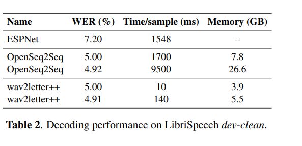
The model was evaluated on the Wall Street Journal (WSJ) dataset. Training time was evaluated using 2 types of neural network architectures: recurrent, with 30 million parameters, and purely convolutional, with 100 million parameters. The figure below shows the Word Error Rate obtained on LibriSpeech.
SpecAugment: A Simple Data Augmentation Method for Automatic Speech Recognition
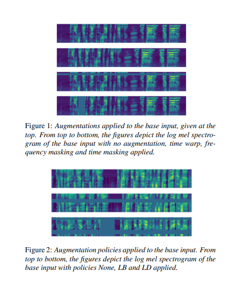
Google Brain authors preset a simple data augmentation method for speech recognition known as SpecAugment. The method operates on the log mel spectrogram of the input audio.
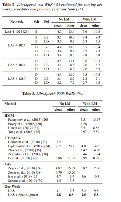
On the LibriSpeech test-other set, the authors achieve a 6.8% WER (Word Error Rate) without a language model, and 5.8% WER with a language model. For Switchboard, they achieve 7.2%/14.6% on the Switchboard/CallHome.
Using this method, the authors are able to train end-to-end ASR (automatic speech recognition) networks known as Listen, Attend and Spell (LAS). The data augmentation policy used involves time warping, frequency masking, and time masking.
In the LAS Networks, the input log mel spectrogram is passed into a 2-layer convolutional neural network (CNN) with a stride of 2. The output of this CNN is passed through an encoder that has d stacked bi-directional LSTMs with cell size w to produce a series of attention vectors.
The attention vectors are fed into a 2-layer RNN decoder of cell dimension w. This outputs the tokens for the transcript. Tokenization of the text is done using a Word Piece Model of 16k for LibriSpeech vocabulary and 1k for Switchboard. The final transcripts are obtained by a beam search with beam size 8.
Here’s the Word Error Rate performance of LAS + SpecAugment.
Wav2Vec: Unsupervised Pre-training for Speech Recognition
Authors from Facebook AI Research explore unsupervised pre-training for speech recognition by learning representations of raw audio. The result is Wav2Vec, a model that’s trained on a huge unlabeled audio dataset.
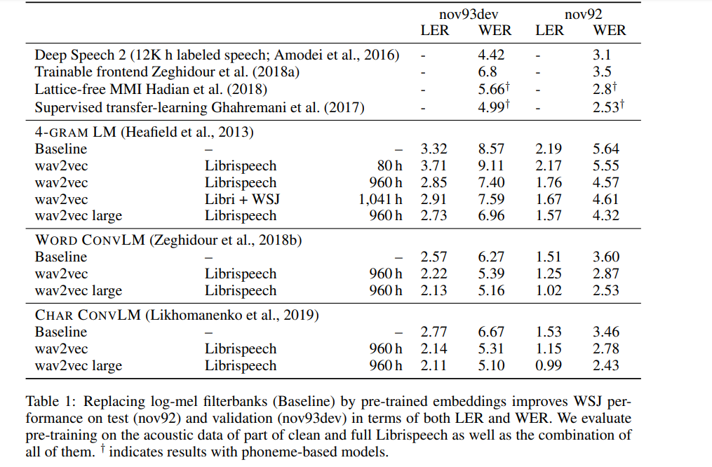
The representations obtained from this are then used to improve acoustic model training. A simple multi-layer convolutional neural network is pre-trained and optimized through a noise contrastive binary classification task. Wav2Vec achieves a 2.43% WER on the nov92 test set.
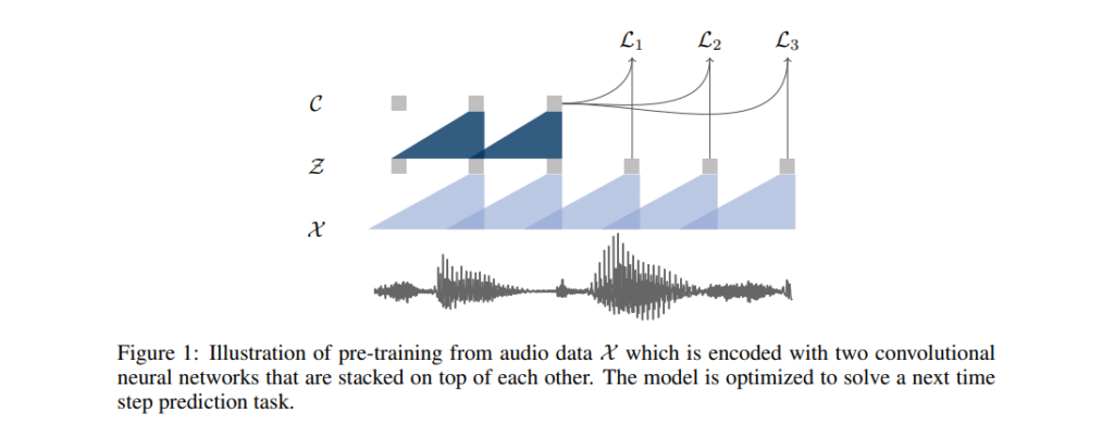
The approach used in pre-training is optimizing the model to predict future samples from a single context. The model takes a raw audio signal as input and then applies an encoder network and a context network.
The encoder network embeds the audio signal in a latent space, and the context network combines multiple time-steps of the encoder to obtain representations that have been contextualized. The objective function is then computed from both networks.
Layers in the encoder and context networks are made up of a causal convolution with 512 channels, a group normalization layer, and a ReLU nonlinearity activation function. The representations produced by the context network during training are fed to the acoustic model. Training and evaluation of acoustic models are done using the wav2letter++ toolkit. For decoding, a lexicon and a separate language model trained on the WSJ language modeling dataset are used.
Here’s the Word Error Rate for this model compared to other speech recognition models.
Scalable Multi Corpora Neural Language Models for ASR
In this paper, authors from Amazon Alexa offer solutions to some of the challenges encountered when using Neural Language Models for large scale ASR systems.
The challenges the authors seek to address are:
- Training the NLM on multiple heterogenous corpora
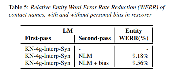
- Personalizing the Neural Language Model(NLM) by passing biases for classes such as contact names from the first-pass model through the NLM
- Incorporating the NLM into the ASR system, while limiting the latency impact
For the task of learning from heterogeneous corpora, parameters of the neural network are estimated using a variant of stochastic gradient descent. This method is dependent upon each minibatch being an Independent and Identically (iid) sample of the distribution that is being learned from. Minibatches are constructed stochastically by drawing samples from each corpus with probability based on its relevance. Constructing n-gram models from each data source and optimizing their linear interpolation weights on a development set is used for relevance weights.
Generating synthetic data for first-pass LM is done by constructing an n-gram approximation of NLM by sampling a large text corpus from NLM and estimating an n-gram model from the corpus. A subword NLM is used to generate synthetic data to ensure that the generated corpus is not limited to the vocabulary of the current version of the ASR system. The written text corpora used in the model contains over 50 billion words in total. The NLM architecture is made up of two Long Short-Term Memory Projection Recurrent Neural Network(LSTMP) layers, each comprising 1024 hidden units projected down to a dimension of 512. There are residual connections between the layers.
Here are some of the results obtained from this model. It obtains a 1.6% relative WERR by generating synthetic data from the NLM.
Conclusion
We should now be up to speed on some of the most common — and a couple of very recent — techniques for performing automatic speech recognition in a variety of contexts.
The papers/abstracts mentioned and linked to above also contain links to their code implementations. We’d be happy to see the results you obtain after testing them.

Comments 0 Responses