Using a Keras Long Short-Term Memory (LSTM) Model to Predict Stock Prices

Editor’s note: This tutorial illustrates how to get started forecasting time series with LSTM models. Stock market data is a great choice for this because it’s quite regular and widely available to everyone. Please don’t take this as financial advice or use it to make any trades of your own.

In this tutorial, we’ll build a Python deep learning model that will predict the future behavior of stock prices. We assume that the reader is familiar with the concepts of deep learning in Python, especially Long Short-Term Memory.

While predicting the actual price of a stock is an uphill climb, we can build a model that will predict whether the price will go up or down. The data and notebook used for this tutorial can be found here. It’s important to note that there are always other factors that affect the prices of stocks, such as the political atmosphere and the market. However, we won’t focus on those factors for this tutorial.

Introduction

LSTMs are very powerful in sequence prediction problems because they’re able to store past information. This is important in our case because the previous price of a stock is crucial in predicting its future price.

We’ll kick of by importing NumPy for scientific computation, Matplotlib for plotting graphs, and Pandas to aide in loading and manipulating our datasets.

import numpy as np
import matplotlib.pyplot as plt
import pandas as pd

Loading the Dataset

The next step is to load in our training dataset and select the Open and High columns that we’ll use in our modeling.

dataset_train = pd.read_csv('NSE-TATAGLOBAL.csv')
training_set = dataset_train.iloc[:, 1:2].values

We check the head of our dataset to give us a glimpse into the kind of dataset we’re working with.

dataset_train.head()

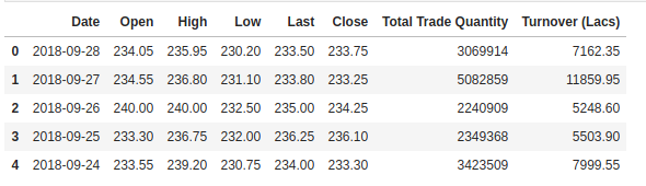
The Open column is the starting price while the Close column is the final price of a stock on a particular trading day. The High and Low columns represent the highest and lowest prices for a certain day.

Feature Scaling

From previous experience with deep learning models, we know that we have to scale our data for optimal performance. In our case, we’ll use Scikit- Learn’s MinMaxScaler and scale our dataset to numbers between zero and one.

from sklearn.preprocessing import MinMaxScaler
sc = MinMaxScaler(feature_range = (0, 1))
training_set_scaled = sc.fit_transform(training_set)

Creating Data with Timesteps

LSTMs expect our data to be in a specific format, usually a 3D array. We start by creating data in 60 timesteps and converting it into an array using NumPy. Next, we convert the data into a 3D dimension array with X_train samples, 60 timestamps, and one feature at each step.

X_train = []
y_train = []
for i in range(60, 2035):
    X_train.append(training_set_scaled[i-60:i, 0])
    y_train.append(training_set_scaled[i, 0])
X_train, y_train = np.array(X_train), np.array(y_train)

X_train = np.reshape(X_train, (X_train.shape[0], X_train.shape[1], 1))

Building the LSTM

In order to build the LSTM, we need to import a couple of modules from Keras:

Sequential for initializing the neural network
Dense for adding a densely connected neural network layer
LSTM for adding the Long Short-Term Memory layer
Dropout for adding dropout layers that prevent overfitting

from keras.models import Sequential
from keras.layers import Dense
from keras.layers import LSTM
from keras.layers import Dropout

We add the LSTM layer and later add a few Dropout layers to prevent overfitting. We add the LSTM layer with the following arguments:

50 units which is the dimensionality of the output space
return_sequences=True which determines whether to return the last output in the output sequence, or the full sequence
input_shape as the shape of our training set.

When defining the Dropout layers, we specify 0.2, meaning that 20% of the layers will be dropped. Thereafter, we add the Dense layer that specifies the output of 1 unit. After this, we compile our model using the popular Adam optimizer and set the loss as the mean_squarred_error. This will compute the mean of the squared errors. Next, we fit the model to run on 100 epochs with a batch size of 32. Keep in mind that, depending on the specs of your computer, this might take a few minutes to finish running.


regressor = Sequential()

regressor.add(LSTM(units = 50, return_sequences = True, input_shape = (X_train.shape[1], 1)))
regressor.add(Dropout(0.2))

regressor.add(LSTM(units = 50, return_sequences = True))
regressor.add(Dropout(0.2))

regressor.add(LSTM(units = 50, return_sequences = True))
regressor.add(Dropout(0.2))

regressor.add(LSTM(units = 50))
regressor.add(Dropout(0.2))

regressor.add(Dense(units = 1))

regressor.compile(optimizer = 'adam', loss = 'mean_squared_error')

regressor.fit(X_train, y_train, epochs = 100, batch_size = 32)

Predicting Future Stock using the Test Set

First we need to import the test set that we’ll use to make our predictions on.

dataset_test = pd.read_csv('tatatest.csv')
real_stock_price = dataset_test.iloc[:, 1:2].values

In order to predict future stock prices we need to do a couple of things after loading in the test set:

Merge the training set and the test set on the 0 axis.
Set the time step as 60 (as seen previously)
Use MinMaxScaler to transform the new dataset
Reshape the dataset as done previously

After making the predictions we use inverse_transform to get back the stock prices in normal readable format.

dataset_total = pd.concat((dataset_train['Open'], dataset_test['Open']), axis = 0)
inputs = dataset_total[len(dataset_total) - len(dataset_test) - 60:].values
inputs = inputs.reshape(-1,1)
inputs = sc.transform(inputs)
X_test = []
for i in range(60, 76):
    X_test.append(inputs[i-60:i, 0])
X_test = np.array(X_test)
X_test = np.reshape(X_test, (X_test.shape[0], X_test.shape[1], 1))
predicted_stock_price = regressor.predict(X_test)
predicted_stock_price = sc.inverse_transform(predicted_stock_price)

Plotting the Results

Finally, we use Matplotlib to visualize the result of the predicted stock price and the real stock price.

plt.plot(real_stock_price, color = 'black', label = 'TATA Stock Price')
plt.plot(predicted_stock_price, color = 'green', label = 'Predicted TATA Stock Price')
plt.title('TATA Stock Price Prediction')
plt.xlabel('Time')
plt.ylabel('TATA Stock Price')
plt.legend()
plt.show()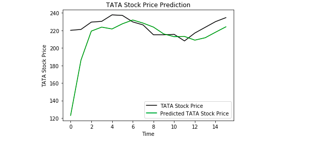

From the plot we can see that the real stock price went up while our model also predicted that the price of the stock will go up. This clearly shows how powerful LSTMs are for analyzing time series and sequential data.

Conclusion

There are a couple of other techniques of predicting stock prices such as moving averages, linear regression, K-Nearest Neighbours, ARIMA and Prophet. These are techniques that one can test on their own and compare their performance with the Keras LSTM. If you wish to learn more about Keras and deep learning you can find my articles on that here and here.

Discuss this post on Reddit and Hacker News.