
Due to the popularity of deep neural networks, many recent hardware platforms have special features that target deep neural network processing. The Intel Knights Mill CPU will feature special vector instructions for deep learning. The Nvidia PASCAL GP100 GPU features 16-b floating-point (FP16) arithmetic support to perform two FP16 operations on a single-precision core for faster deep learning computation.
Systems have also been built specifically for DNN processing, such as the Nvidia DGX-1 and Facebook’s Big Basin custom DNN server. DNN inference has also been demonstrated on various embedded System-on-Chips (SoCs) such as Nvidia Tegra and Samsung Exynos, as well as on field-programmable gate arrays (FPGAs).
Accordingly, it’s important to have a good understanding of how the processing of neural networks is being performed on these platforms, and how application-specific accelerators can be designed for deep neural networks for further improvement in throughput and energy efficiency.
The fundamental component of both the convolution and fully-connected layers are the multiply-and-accumulate (MAC) operations, which can be easily parallelized. In order to achieve high performance, highly-parallel computing paradigms are commonly used, including both temporal and spatial architectures, as shown below:
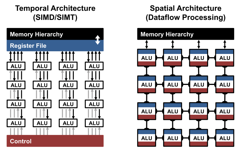
The temporal architectures appear mostly in CPUs or GPUs and employ a variety of techniques to improve parallelisms, such as vectors (SIMD) or parallel threads (SIMT). Such temporal architectures use a centralized control for a large number of arithmetic logic units (ALUs). These ALUs can only fetch data from the memory hierarchy and cannot communicate directly with each other.
In contrast, spatial architectures use dataflow processing; i.e., the ALUs form a processing chain so that they can pass data from one to another directly. Sometimes each ALU can have its own control logic and local memory called a scratchpad or register file. We refer to the ALU with its own local memory as a processing engine (PE). Spatial architectures are commonly used for deep neural networks in ASIC and FPGA-based designs.
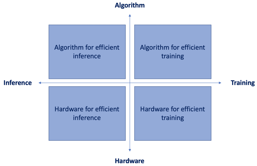
In the previous articles in Heartbeat, I addressed different algorithms for efficient inference and efficient training. In this article, I’ll tackle the lower row of the quadrant below by discussing the different design strategies for efficient inference/training on these different hardware platforms, specifically:
- For temporal architectures such as CPUs and GPUs, I’ll discuss how computational transforms on the kernel can reduce the number of multiplications to increase throughput.
- For spatial architectures used in accelerators, I will discuss how dataflows can increase data reuse from low-cost memories in the memory hierarchy to reduce energy consumption.
1 — Temporal Hardware Architectures
CPUs and GPUs use parallelization techniques to perform the multiply-and-accumulate operations in parallel. All the ALUs share the same control and memory (register file). On these platforms, both the fully-connected and convolution layers are often mapped to a matrix multiplication (i.e., the kernel computation).
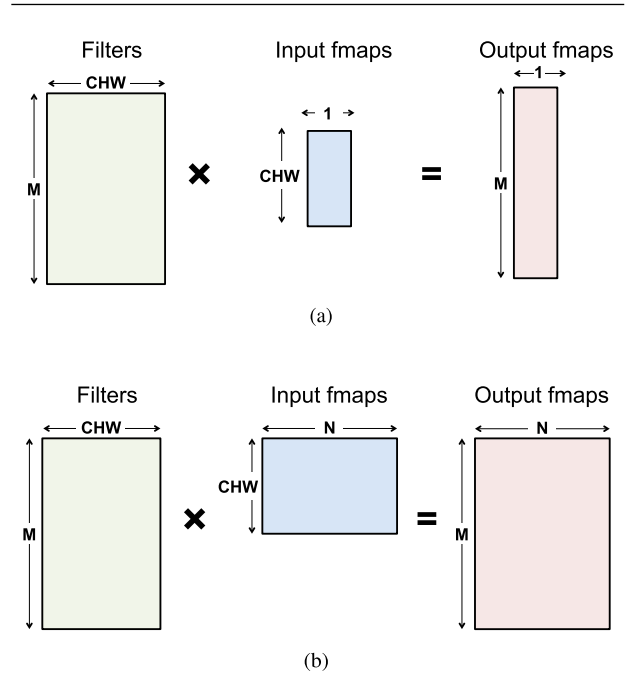
The figure to the left shows how matrix multiplication is used for the fully-connected layer.
- The height of the filter matrix is the number of 3D filters, and the width is the number of weights per 3D filter.
- The height of the input feature map’s matrix is the number of activations per 3D input feature map (C × W × H), and the width is the number of 3D input feature maps.
- Finally, the height of the output feature map matrix is the number of channels in the output feature maps (M), and the width is the number of 3D output feature maps (N), where each output feature map of the FC layer has the dimension of 1 × 1 ×number of output channels (M).
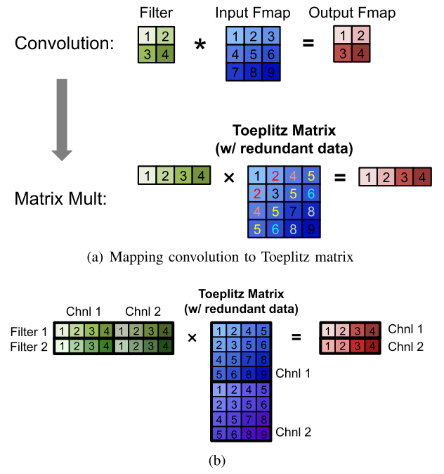
The convolution layer in a deep neural network can also be mapped to a matrix multiplication using a relaxed form of the Toeplitz matrix, as shown below. The downside of using matrix multiplication for the convolution layers is that there is redundant data in the input feature map matrix, as highlighted. This can lead to either inefficiency in storage, or a complex memory access pattern.
There are software libraries designed for CPUs (e.g., OpenBLAS, Intel MKL, etc.) and GPUs (e.g., cuBLAS, cuDNN, etc.) that optimize for matrix multiplications. The matrix multiplication is tiled to the storage hierarchy of these platforms, which are on the order of a few megabytes at the higher levels.
The matrix multiplications on these platforms can be further sped up by applying computational transforms to the data to reduce the number of multiplications, while still giving the same bitwise result. Often this can come at a cost of an increased number of additions and a more irregular data access pattern.
Fast Fourier transform (FFT) is a well-known approach (shown below). To perform the convolution, we take the FFT of the filter and input feature map, and then perform the multiplication in the frequency domain; we then apply an inverse FFT to the resulting product to recover the output feature map in the spatial domain.
However, there are several drawbacks to using FFT: 1) the benefits of FFTs decrease with filter size, 2) the size of the FFT is dictated by the output feature map size, which is often much larger than the filter, and 3) the coefficients in the frequency domain are complex. As a result, while FFT reduces computation, it requires more storage capacity and bandwidth.
Finally, a popular approach for reducing complexity is to make the weights sparse; using FFTs makes it difficult for this sparsity to be exploited.
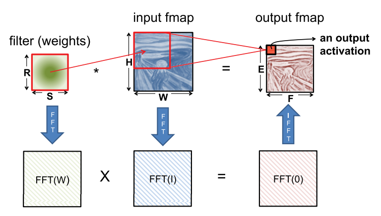
Several optimizations can be performed on FFT to make it more effective for DNNs. To reduce the number of operations, the FFT of the filter can be precomputed and stored. In addition, the FFT of the input feature map can be computed once and used to generate multiple channels in the output feature map. Finally, since an image contains only real values, its Fourier transform is symmetric, and this can be exploited to reduce storage and computation costs.
Similar to FFT, Winograd’s algorithm applies transforms to the feature map and filter to reduce the number of multiplications required for convolution. Winograd is applied on a block-by-block basis, and the reduction in multiplications varies based on the filter and block size. A larger block size results in a larger reduction in multiplies at the cost of higher complexity transforms. A particularly attractive filter size is 3 × 3, which can reduce the number of multiplications by 2.25× when computing a block of 2 × 2 outputs. Note that Winograd requires specialized processing depending on the size of the filter and block.
Strassen’s algorithm has also been explored for reducing the number of multiplications in deep neural networks. It rearranges the computations of a matrix multiplication in a recursive manner to reduce the number of multiplications from O(N³) to O(N².807). However, Strassen’s benefits come at the cost of increased storage requirements and sometimes reduced numerical stability. In practice, different algorithms might be used for different layer shapes and sizes (e.g., FFT for filters greater than 5 × 5, and Winograd for filters 3 × 3 and below). Existing platform libraries, such as Intel’s Math Kernel Library and NVIDIA’s cuDNN, can dynamically choose the appropriate algorithm for a given shape and size.
2 — Spatial Hardware Architectures
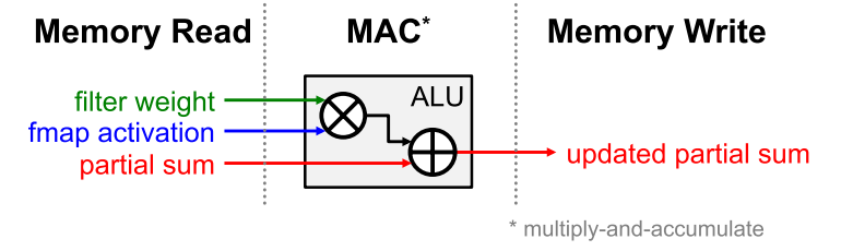
For deep neural networks, the bottleneck for processing is in the memory access. Each MAC requires three memory reads (for filter weight, fmap activation, and partial sum) and one memory write (for the updated partial sum), as shown below.
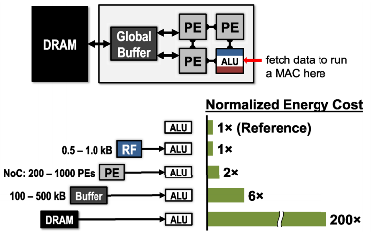
In the worst case, all of the memory accesses have to go through the off-chip DRAM, which will severely impact both throughput and energy efficiency. For example, in AlexNet, to support its 724 million MACs, nearly 3000 million DRAM accesses will be required. Furthermore, DRAM accesses require up to several orders of magnitude higher energy than computation.
Accelerators provide an opportunity to reduce the energy cost of data movement by introducing several levels of local memory hierarchy with different energy costs, as shown below. This includes a large global buffer with a size of several hundred kilobytes that connects to DRAM, an inter-PE network that can pass data directly between the ALUs, and a register file (RF) within each processing element (PE) with a size of a few kilobytes or less.
The multiple levels of memory hierarchy help to improve energy efficiency by providing low-cost data accesses. For example, fetching the data from the RF or neighbor PEs is going to cost one or two orders of magnitude lower in terms of energy than fetching from DRAM.
Accelerators can be designed to support specialized processing dataflows that leverage this memory hierarchy. The dataflow decides what data get read into which level of the memory hierarchy and when they end up getting processed.
Since there’s no randomness in the processing of deep neural networks, it’s possible to design a fixed dataflow that can adapt to the neural network shapes and sizes and optimize for energy efficiency. The optimized dataflow minimizes access from the more energy-consuming levels of the memory hierarchy.
Large memories that can store a significant amount of data consume more energy than smaller memories. For instance, DRAM can store gigabytes of data but consumes two orders of magnitude higher energy per access than a small on-chip memory of a few kilobytes. Thus, every time a piece of data is moved from an expensive level to a lower-cost level in terms of energy, we want to reuse that piece of data as much as possible to minimize subsequent accesses to the expensive levels.
The challenge, however, is that the storage capacity of these low-cost memories is limited. Thus we need to explore different dataflows that maximize reuse under these constraints.
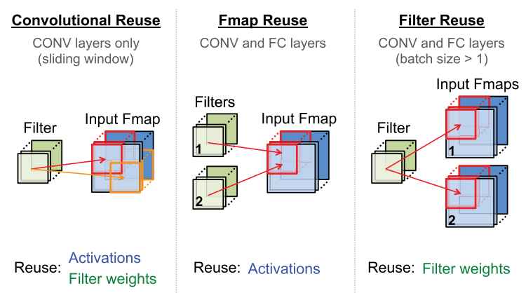
For deep neural networks, we investigate dataflows that exploit three forms of input data reuse (convolutional, feature map, and filter), as shown below. For convolutional reuse, the same input feature map activations and filter weights are used within a given channel, just in different combinations for different weighted sums.
For feature map reuse, multiple filters are applied to the same feature map, so the input feature map activations are used multiple times across filters. Finally, for filter reuse, when multiple input feature maps are processed at once (referred to as a batch), the same filter weights are used multiple times across input features maps.
If we can harness the three types of data reuse by storing the data in the local memory hierarchy and accessing them multiple times without going back to the DRAM, it can save a significant amount of DRAM accesses.
For example, in AlexNet, the number of DRAM reads can be reduced by up to 500× in the CONV layers. The local memory can also be used for partial sum accumulation, so they don’t have to reach DRAM. In the best case, if all data reuse and accumulation can be achieved by the local memory hierarchy, the 3000 million DRAM accesses in AlexNet can be reduced to only 61 million.
Conclusion
The use of deep neural networks has seen explosive growth in the past few years. They are currently widely used for many AI applications, including computer vision, speech recognition, and robotics, and are often delivering better-than-human accuracy.
However, while deep neural networks can deliver this outstanding accuracy, it comes at the cost of high computational complexity. Consequently, techniques that enable efficient processing of deep neural networks to improve energy efficiency and throughput without sacrificing accuracy with cost-effective hardware are critical to expanding the deployment of deep neural networks in both existing and new domains.
Creating a system for efficient deep neural network processing should begin with understanding the current and future applications and the specific computations require—both for now and for the potential evolution of those computations.
This post in particular surveys a number of avenues that prior work has taken to optimize deep neural network processing. Since data movement dominates energy consumption, a primary focus of some recent research has been to reduce data movement while maintaining accuracy, throughput, and cost. This means selecting architectures with favorable memory hierarchies like a spatial array and developing dataflows that increase data reuse at the low-cost levels of the memory hierarchy.

Comments 0 Responses