5 Regression Loss Functions All Machine Learners Should Know

All the algorithms in machine learning rely on minimizing or maximizing a function, which we call “objective function”. The group of functions that are minimized are called “loss functions”. A loss function is a measure of how good a prediction model does in terms of being able to predict the expected outcome. A most commonly used method of finding the minimum point of function is “gradient descent”. Think of loss function like undulating mountain and gradient descent is like sliding down the mountain to reach the bottommost point.

There is not a single loss function that works for all kind of data. It depends on a number of factors including the presence of outliers, choice of machine learning algorithm, time efficiency of gradient descent, ease of finding the derivatives and confidence of predictions. The purpose of this blog series is to learn about different losses and how each of them can help data scientists.

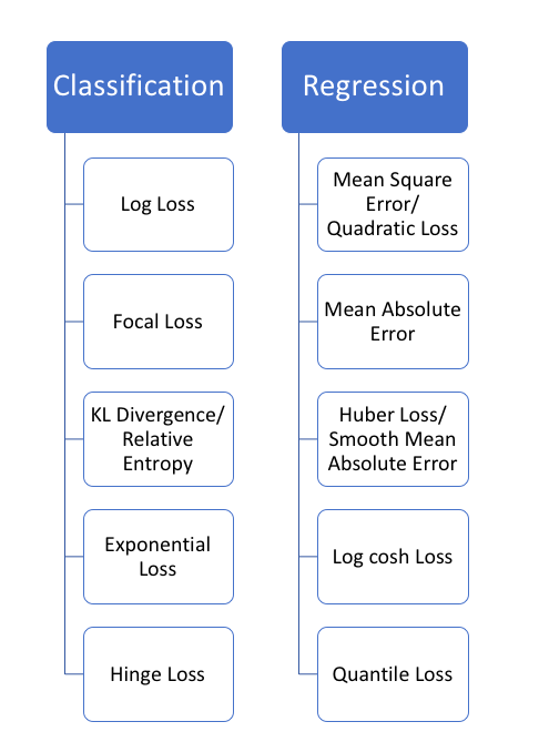
Loss functions can be broadly categorized into 2 types: Classification and Regression Loss. In this post, I’m focussing on regression loss. In future posts I cover loss functions in other categories. Please let me know in comments if I miss something. Also, all the codes and plots shown in this blog can be found in this notebook.

Regression loss

1. Mean Square Error, Quadratic loss, L2 Loss

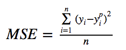
Mean Square Error (MSE) is the most commonly used regression loss function. MSE is the sum of squared distances between our target variable and predicted values.

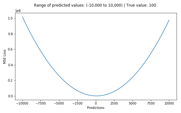
Below is a plot of an MSE function where the true target value is 100, and the predicted values range between -10,000 to 10,000. The MSE loss (Y-axis) reaches its minimum value at prediction (X-axis) = 100. The range is 0 to ∞.

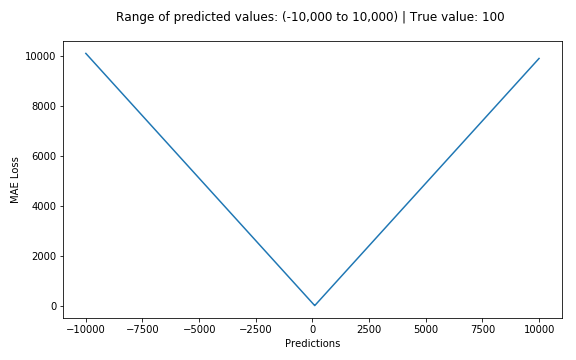
2. Mean Absolute Error, L1 Loss

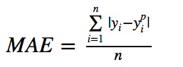
Mean Absolute Error (MAE) is another loss function used for regression models. MAE is the sum of absolute differences between our target and predicted variables. So it measures the average magnitude of errors in a set of predictions, without considering their directions. (If we consider directions also, that would be called Mean Bias Error (MBE), which is a sum of residuals/errors). The range is also 0 to ∞.

MSE vs. MAE (L2 loss vs L1 loss)

In short, using the squared error is easier to solve, but using the absolute error is more robust to outliers. But let’s understand why!

Whenever we train a machine learning model, our goal is to find the point that minimizes loss function. Of course, both functions reach the minimum when the prediction is exactly equal to the true value.

Here’s a quick review of python code for both. We can either write our own functions or use sklearn’s built-in metrics functions:

# true: Array of true target variable
# pred: Array of predictions

def mse(true, pred): 
    return np.sum((true - pred)**2)
    
 def mae(true, pred):
  return np.sum(np.abs(true - pred))
 
 # also available in sklearn
 
 from sklearn.metrics import mean_squared_error
 from sklearn.metrics import mean_absolute_error

Let’s see the values of MAE and Root Mean Square Error (RMSE, which is just the square root of MSE to make it on the same scale as MAE) for 2 cases. In the first case, the predictions are close to true values and the error has small variance among observations. In the second, there is one outlier observation, and the error is high.

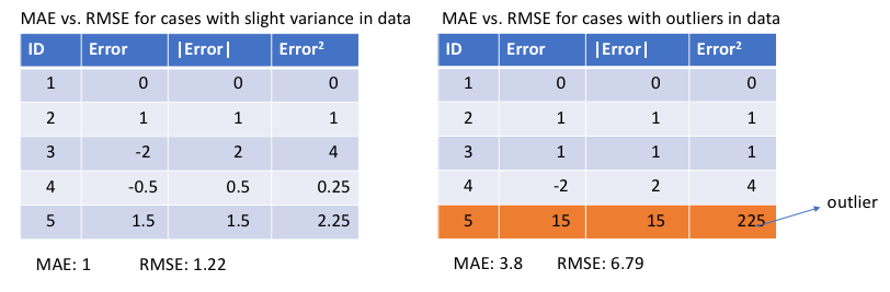
What do we observe from this, and how can it help us to choose which loss function to use?

Since MSE squares the error (y — y_predicted = e), the value of error (e) increases a lot if e > 1. If we have an outlier in our data, the value of e will be high and e² will be >> |e|. This will make the model with MSE loss give more weight to outliers than a model with MAE loss. In the 2nd case above, the model with RMSE as loss will be adjusted to minimize that single outlier case at the expense of other common examples, which will reduce its overall performance.

MAE loss is useful if the training data is corrupted with outliers (i.e. we erroneously receive unrealistically huge negative/positive values in our training environment, but not our testing environment).

Intuitively, we can think about it like this: If we only had to give one prediction for all the observations that try to minimize MSE, then that prediction should be the mean of all target values. But if we try to minimize MAE, that prediction would be the median of all observations. We know that median is more robust to outliers than mean, which consequently makes MAE more robust to outliers than MSE.

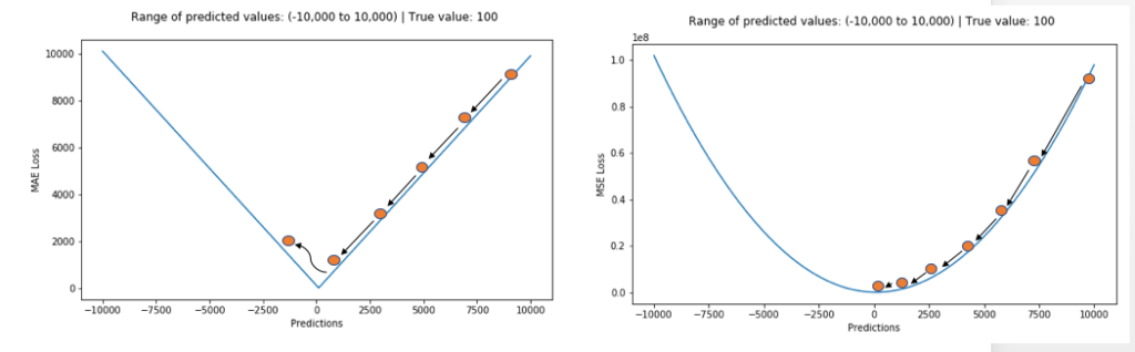
One big problem in using MAE loss (for neural nets especially) is that its gradient is the same throughout, which means the gradient will be large even for small loss values. This isn’t good for learning. To fix this, we can use dynamic learning rate which decreases as we move closer to the minima. MSE behaves nicely in this case and will converge even with a fixed learning rate. The gradient of MSE loss is high for larger loss values and decreases as loss approaches 0, making it more precise at the end of training (see figure below.)

Deciding which loss function to use
If the outliers represent anomalies that are important for business and should be detected, then we should use MSE. On the other hand, if we believe that the outliers just represent corrupted data, then we should choose MAE as loss.

I recommend reading this post with a nice study comparing the performance of a regression model using L1 loss and L2 loss in both the presence and absence of outliers. Remember, L1 and L2 loss are just another names for MAE and MSE respectively.

Problems with both: There can be cases where neither loss function gives desirable predictions. For example, if 90% of observations in our data have true target value of 150 and the remaining 10% have target value between 0–30. Then a model with MAE as loss might predict 150 for all observations, ignoring 10% of outlier cases, as it will try to go towards median value. In the same case, a model using MSE would give many predictions in the range of 0 to 30 as it will get skewed towards outliers. Both results are undesirable in many business cases.

What to do in such a case? An easy fix would be to transform the target variables. Another way is to try a different loss function. This is the motivation behind our 3rd loss function, Huber loss.

3. Huber Loss, Smooth Mean Absolute Error

Huber loss is less sensitive to outliers in data than the squared error loss. It’s also differentiable at 0. It’s basically absolute error, which becomes quadratic when error is small. How small that error has to be to make it quadratic depends on a hyperparameter, 𝛿 (delta), which can be tuned. Huber loss approaches MSE when 𝛿 ~ 0 and MAE when 𝛿 ~ ∞ (large numbers.)

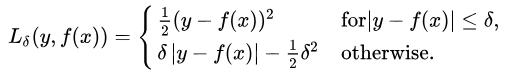
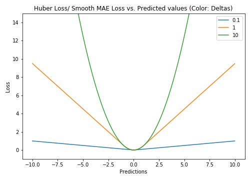
The choice of delta is critical because it determines what you’re willing to consider as an outlier. Residuals larger than delta are minimized with L1 (which is less sensitive to large outliers), while residuals smaller than delta are minimized “appropriately” with L2.

Why use Huber Loss?
One big problem with using MAE for training of neural nets is its constantly large gradient, which can lead to missing minima at the end of training using gradient descent. For MSE, gradient decreases as the loss gets close to its minima, making it more precise.

Huber loss can be really helpful in such cases, as it curves around the minima which decreases the gradient. And it’s more robust to outliers than MSE. Therefore, it combines good properties from both MSE and MAE. However, the problem with Huber loss is that we might need to train hyperparameter delta which is an iterative process.

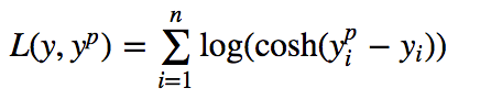
4. Log-Cosh Loss

Log-cosh is another function used in regression tasks that’s smoother than L2. Log-cosh is the logarithm of the hyperbolic cosine of the prediction error.

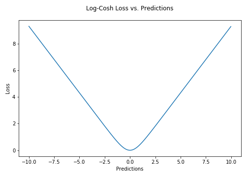
Advantage: log(cosh(x)) is approximately equal to (x ** 2) / 2 for small x and to abs(x) – log(2) for large x. This means that ‘logcosh’ works mostly like the mean squared error, but will not be so strongly affected by the occasional wildly incorrect prediction. It has all the advantages of Huber loss, and it’s twice differentiable everywhere, unlike Huber loss.

Why do we need a 2nd derivative? Many ML model implementations like XGBoost use Newton’s method to find the optimum, which is why the second derivative (Hessian) is needed. For ML frameworks like XGBoost, twice differentiable functions are more favorable.

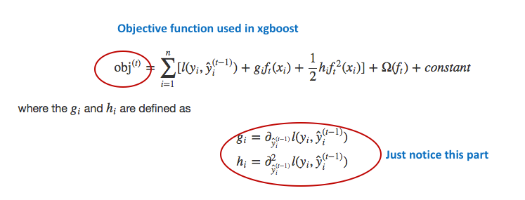
But Log-cosh loss isn’t perfect. It still suffers from the problem of gradient and hessian for very large off-target predictions being constant, therefore resulting in the absence of splits for XGBoost.

Python code for Huber and Log-cosh loss functions:

# huber loss
def huber(true, pred, delta):
    loss = np.where(np.abs(true-pred) < delta , 0.5*((true-pred)**2), delta*np.abs(true - pred) - 0.5*(delta**2))
    return np.sum(loss)

# log cosh loss
def logcosh(true, pred):
    loss = np.log(np.cosh(pred - true))
    return np.sum(loss)

5. Quantile Loss

In most of the real-world prediction problems, we are often interested to know about the uncertainty in our predictions. Knowing about the range of predictions as opposed to only point estimates can significantly improve decision making processes for many business problems.

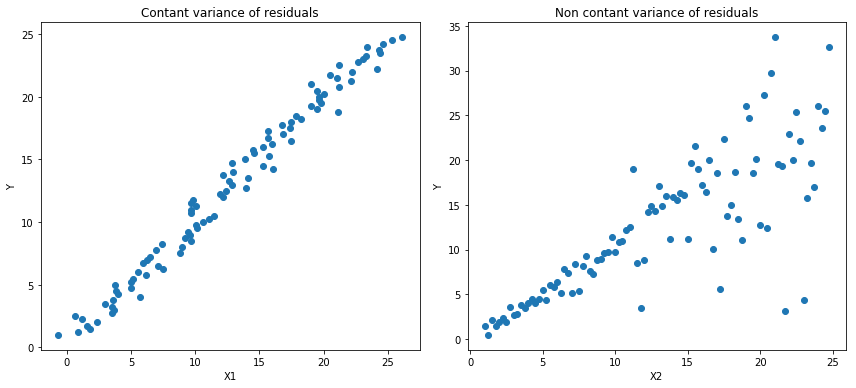
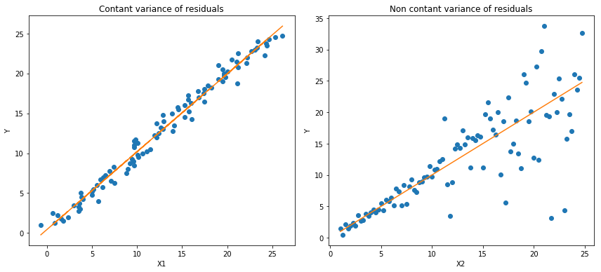
Quantile loss functions turn out to be useful when we are interested in predicting an interval instead of only point predictions. Prediction interval from least square regression is based on an assumption that residuals (y — y_hat) have constant variance across values of independent variables. We can not trust linear regression models that violate this assumption. We can not also just throw away the idea of fitting a linear regression model as the baseline by saying that such situations would always be better modeled using non-linear functions or tree-based models. This is where quantile loss and quantile regression come to the rescue as regression-based on quantile loss provides sensible prediction intervals even for residuals with non-constant variance or non-normal distribution.

Let’s see a working example to better understand why regression based on quantile loss performs well with heteroscedastic data.

Quantile regression vs. Ordinary Least Square regression

Notebook link with codes for quantile regression shown in the above plots.

Understanding the quantile loss function

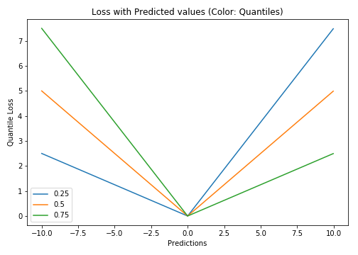
Quantile-based regression aims to estimate the conditional “quantile” of a response variable given certain values of predictor variables. Quantile loss is actually just an extension of MAE (when the quantile is 50th percentile, it is MAE).

The idea is to choose the quantile value based on whether we want to give more value to positive errors or negative errors. Loss function tries to give different penalties to overestimation and underestimation based on the value of the chosen quantile (γ). For example, a quantile loss function of γ = 0.25 gives more penalty to overestimation and tries to keep prediction values a little below median

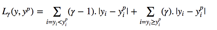
γ is the required quantile and has value between 0 and 1.

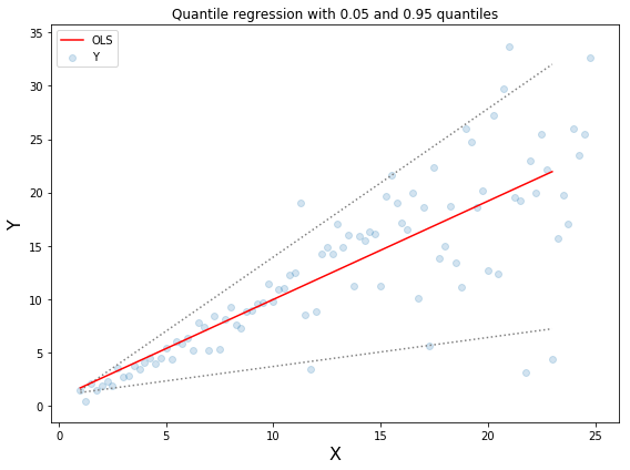
We can also use this loss function to calculate prediction intervals in neural nets or tree based models. Below is an example of Sklearn implementation for gradient boosted tree regressors.

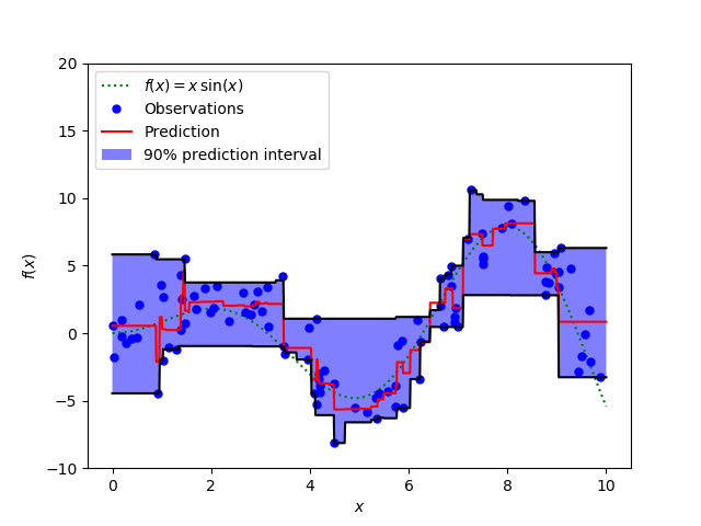
The above figure shows a 90% prediction interval calculated using the quantile loss function available in GradientBoostingRegression of sklearn library. The upper bound is constructed γ = 0.95 and lower bound using γ = 0.05.

___________________________________________________________________

Comparison Study:

A nice comparison simulation is provided in “Gradient boosting machines, a tutorial”. To demonstrate the properties of all the above loss functions, they’ve simulated a dataset sampled from a sinc(x) function with two sources of artificially simulated noise: the Gaussian noise component ε ~ N(0, σ2) and the impulsive noise component ξ ~ Bern(p). The impulsive noise term is added to illustrate the robustness effects. Below are the results of fitting a GBM regressor using different loss functions.

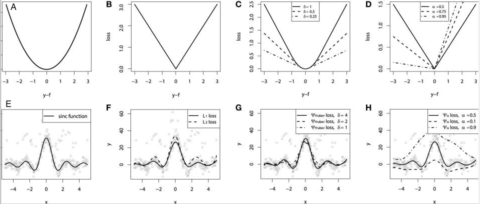
Some observations from the simulations:

The predictions from the model with MAE loss are less affected by the impulsive noise whereas the predictions with MSE loss function are slightly biased due to the caused deviations.
The predictions are little sensitive to the value of hyperparameter chosen in the case of the model with Huber loss.
The quantile losses give a good estimation of the corresponding confidence levels.

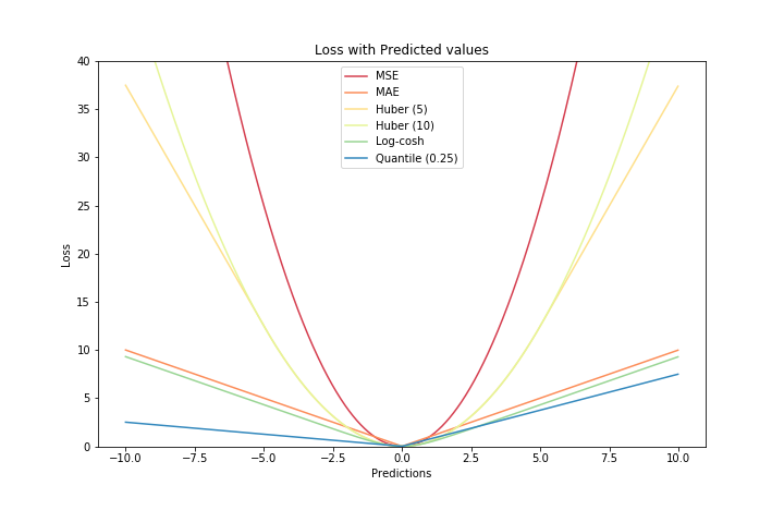
All the loss functions in a single plot.

If I have missed any important loss functions, I would love to hear about them in the comments. Thank you for reading.

LinkedIn: https://www.linkedin.com/in/groverpr/

References:

Discuss this post on Hacker News.